Exercise 2.5.6. Determine the incidence matrix  for the graph on page 113 with six edges and four nodes, as follows: Edge 1 from node 1 to node 2, edge 2 from node 1 to node 3, edge 3 from node 2 to node 3, edge 4 from node 2 to node 4, edge 5 from node 1 to node 4, and edge 6 from node 3 to node 4.
Find three independent vectors  that satisfy
  . How do these vectors relate to the loops in the graph?
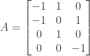
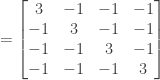
Answer: Since there are six edges in the graph the incidence matrix has six rows, and since there are four nodes has four columns; is therefore a 6 by 4 matrix.
The first row of corresponds to edge 1. Since edge 1 goes from node 1 to node 2 the entry in the (1, 1) position is -1 (representing “flow” out of node 1) and the entry in the (1, 2) position is 1 (representing flow into node 2). Since edge 2 goes from node 1 to node 3 the entry in the (2, 1) position is -1 (representing flow out of node 1) and the entry in the (2, 3) position is 1 (representing flow into node 3). The values of the entries for the other rows (edges) can be similarly determined, and the final incidence matrix is

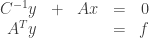
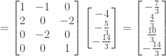
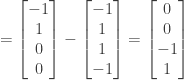
We now try to find a solution to or

by doing Gaussian elimination on  .
.
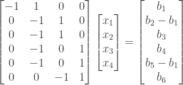
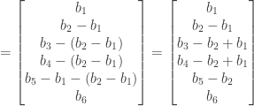
We first subtract -1 times the first row from the second row:
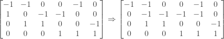
We then subtract -1 times the second row from the third row:
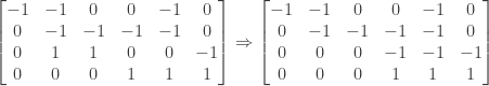
Finally, we subtract -1 times the third row from the fourth row:
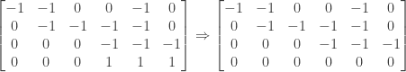
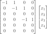
The resulting echelon matrix has pivots in columns one, two, and four, so  ,
,  , and
, and  are basic variables and
  ,
,  , and
, and  are free variables.
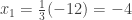
We first set  and
and  . From the third row of the echelon matrix we have


From the second row of the echelon matrix we have


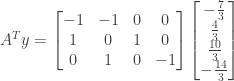
and from the first row we then have


So one solution to is  .
.
We next set  and
and  . From the third row of the echelon matrix we have


From the second row of the echelon matrix we have


and from the first row we then have


So a second solution to is  .
.
Finally we set  and
and  . From the third row of the echelon matrix we have

From the second row of the echelon matrix we have


and from the first row we then have

So a third solution to is 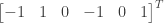 .
.
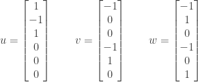
The following set of three vectors  ,
,  , and
, and  are thus solutions to . The vectors are independent (as you can verify by inspecting them):
Since  the vectors are in the left nullspace of . (In fact they form a basis for the left nullspace.)
The vectors also correspond to independent loops in the graph used to create the incidence matrix :
The first vector is a loop around the outside of the graph, and includes edge 1, edge 2, and edge 3. Note that edge 2 runs in a different direction than the other two, and hence its corresponding entry is reversed in sign from the other two.
The second vector is a loop around an interior triangle of the graph (in the upper left), and includes edge 1, edge 4, and edge 5, with edge 5 running in a different direction than the other two.
The third vector includes edges 1, 2, 4, and 6, with edges 2 and 6 running in different directions than the other two.
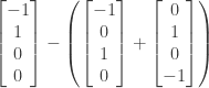
Note that if we add and
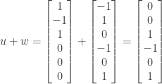
we get a vector representing a loop around the bottom interior triangle of the graph, comprising edges 3, 4, and 6.
Similarly, if we subtract from

we get a vector representing the loop around the upper right interior triangle, comprising edges 2, 5, and 6.
These two vectors together with thus represent independent loops associated with the three interior triangles of the graph.
NOTE: This continues a series of posts containing worked out exercises from the (out of print) book Linear Algebra and Its Applications, Third Edition by Gilbert Strang.
If you find these posts useful I encourage you to also check out the more current Linear Algebra and Its Applications, Fourth Edition , Dr Strang’s introductory textbook Introduction to Linear Algebra, Fourth Edition
 and the accompanying free online course, and Dr Strang’s other books
 .
.
 Buy me a snack to sponsor more posts like this!


 .
.
 and
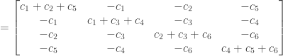
and  . Describe how the diagonal and other entries in


 through
  in
in  for the (1, 1) entry reflects the fact that edges 1, 2, and 5 all have node 1 as an endpoint. The value of
  for the (1, 2) entry reflects the fact that edge 1 connects node 1 to node 2, the value of
  for the (1, 3) entry reflects the fact that edge 2 connects node 1 to node 3, and the value of
  for the (1, 4) entry reflects the fact that edge 5 connects node 1 to node 4.
 to node
  and thus produces an (i, j) entry of the matrix then that same edge also connects node
  :
:
 is therefore 3. The rank is the dimension of the column space of
  the dimension of
  is also 3. The first, second, and third columns of
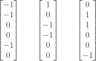
 is 4, the dimension of the nullspace
  is
is  . Since the sum of the columns of
 and forms a basis for
  . The row space of
 and therefore for the rowspace
  is 6, the dimension of the left nullspace
  is
is  .
.
 and are therefore in the left nullspace
  through
  . When you can assign potentials to the teams so that the potentials agree with the values of
  solvable. These can be found via elimination or by using Kirchoff’s Laws.)
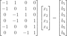


 . From the fifth row we must have
  . Finally, from the sixth row we must have
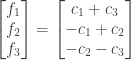
  . Rearranging the terms to put them in order and multiplying the second and third equations by -1 gives us the following three conditions:
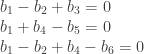
 , and
, and  are the potential differences along each edge, and the sum of the potential differences around the loop must be zero, we must have
 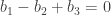 . This gives us the first condition listed above.
 , and
, and  are the potential differences along each edge, and the sum of the potential differences around the loop must be zero, we must have
  . This gives us the second condition listed above.
 . This gives us the third and final condition listed above.
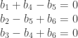


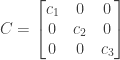


 and
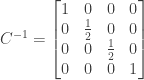
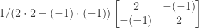
and  as discussed below); its inverse is

 then the 2 by 2 matrix is singular and has no inverse. This would be true, for example, if
  and
and  so that the 2 by 2 matrix derived from


 and subtracting it from the second and third rows:

 ).
). we have
  and
and 
 and substituting into the first equation we have
  . The nullspace therefore consists of all vectors of the form
  . It has dimension
  .
.

 in the row space of
  . Prove the same result based on the linear system
  ,
,  , and
, and  are currents into each node?
 is in the row space of


 in the column space of
  . Prove the same result based on the rows of
  is in the column space of


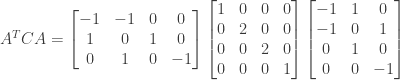
 represents potentials at the nodes (
 is the potential difference along edge 1 (from node 2 to node 1),
  is the potential difference along edge 2 (from node 3 to node 2) and
  is the potential difference along edge 3 (from node 3 to node 1). From the equations above we see that the sum of the potential differences around the loop is zero (Kirchoff‘s Voltage Law).
