Exercise 3.2.16. a) Given the projection matrix  projecting vectors onto the line through
  and two vectors
  and
and  , show that the inner products of with
  and with
  are equal.
b) In general would the angles between and and and be equal to each other? If  ,
,  , and
, and  what are the cosines of the two angles?
c) Show that the inner product of and is the same as the inner products of with and with and explain why this is. What is the angle between the vectors and ?
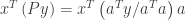
Answer: a) We have  so that

and

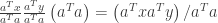
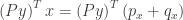
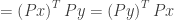
The inner product of with is then


and the inner product of with is then


So the inner products of with and with are equal.
b) Since and are arbitrary vectors, in general they would not make the same angle with respect to . For example, consider the case when , , and .
If  is the angle between and then
  . Similarly, if
  is the angle between and then
In this case we have


So  and
and  . The two cosines are different and thus and are not equal to each other.
c) As noted above we have  and
and  . Their inner product is then

But this is the same as the inner products  and
and  of with and with respectively.
This can be understood geometrically as follows: The vector can be thought of as consisting of two components  and
and  where is the projection of onto and is the projection of onto the vector
  that is orthogonal to . The inner product between and is then

But is simply . Also, since is a projection on and is a projection onto their inner product is zero since is orthogonal to . We therefore have  .
.
Similarly the vector can be thought of as consisting of two components  parallel to and
  orthogonal to , with the inner product between and then being


We thus have  .
.
Since and are both projections onto the angle between them is zero.
NOTE: This continues a series of posts containing worked out exercises from the (out of print) book Linear Algebra and Its Applications, Third Edition by Gilbert Strang.
If you find these posts useful I encourage you to also check out the more current Linear Algebra and Its Applications, Fourth Edition , Dr Strang’s introductory textbook Introduction to Linear Algebra, Fourth Edition
 and the accompanying free online course, and Dr Strang’s other books
 .
.
 Buy me a snack to sponsor more posts like this!


 and
and  find the least squares solution
  and describe the error
  being minimized by that solution. Confirm that the error vector
 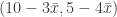 is orthogonal to the column
  .
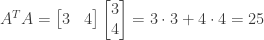
. where
where  and
and  . We can then compute the least squares solution as
 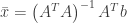 .
.
 . We then have

 .
.

 and the column
  is
is  . Since the inner product is zero the two vectors are orthogonal.
 then the length of
  is equal to the length of
  for all
  . By the rule for transposes of products we have
  so that
  . But since we assumed that
 so that
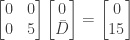
 the planes corresponding to the equations
  and
and  intersect in a line. What is the projection matrix
  where
where

 has pivots in columns 1 and 2 we have
  as a free variable. Setting
  from the second row of
  or
or  . From the first row of
  or
or  . So
. So  is a solution to the system, as is any other vector on the line through the origin and
  is then

 the diagonal entries of
  ,
,  , through
  so that the trace of
 onto the line described by the equation
  .
. . The projection matrix that projects vectors onto the line through

 find the matrix
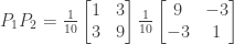
  that projects onto this line, as well as the matrix
  that projects onto the line perpendicular to the original line.
 ? What is
  ? Explain your answers.
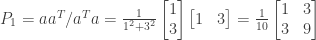
 then we will have
  . One vector satisfying this condition is
  . We then have

 for the same reason.)


 into two perpendicular component vectors: one component
  on the line through
  on the perpendicular line through
  and
and  when calculating the projection matrices. Thanks go to Trystyn for catching my original error.

 of the resulting matrix is equal to the original vector
  multiplied by a scalar factor equal to
  . The columns are therefore linearly dependent with each of them expressible as the first column times the factor
  , and thus the rank of the projection matrix
  . Since the rank
  the matrix
  .
. is a scalar (the inner product of
  is a matrix. We have


