Exercise 3.2.1. a) Consider the vectors  and
and  where
where  and
and  are arbitrary positive real numbers. Use the Schwarz inequality involving
  and
and  to derive a relationship between the arithmetic mean
  and the geometric mean
  .
.
b) Consider a vector from the origin to point , a second vector of length  from to the point
  and the third vector from the origin to . Using the triangle inequality

derive the Schwarz inequality. (Hint: Square both sides of the inequality and expand the expression  .)
.)
Answer: a) From the Schwarz inequality we have

From the definitions of and , on the left side of the inequality we have


assuming we always choose the positive square root.
From the definitions of and we also have

and

so that the right side of the inequality is

again assuming we choose the positive square root. (We know is positive since both and are.)
The Schwartz inequality
then becomes

or (dividing both sides by 2)
We thus see that for any positive real numbers and the geometric mean is less than the arithmetic mean .
b) From the triangle inequality we have
for the vectors and . Squaring the term on the left side of the inequality and using the commutative and distributive properties of the inner product we obtain


Squaring the term on the right side of the inequality we have

The inequality
is thus equivalent to the inequality

Subtracting  and
and  from both sides of the inequality gives us

and dividing both sides of the inequality by 2 produces

Note that this is almost but not quite the Schwarz inequality: Since the Schwarz inequality involves the absolute value  we must also prove that

(After all, the inner product  might be negative, in which case the inequality would be trivially true, given that the term on the right side of the inequality is guaranteed to be positive.)
We have  . Since the triangle inequality holds for any two vectors we can restate it in terms of
  and as follows:

Since  squaring the term on the right side of the inequality produces

as it did previously. However squaring the term on the left side of the inequality produces


The original triangle inequality
is thus equivalent to

or
Since we have both and we therefore have

which is the Schwarz inequality.
So the triangle inequality implies the Schwarz inequality.
NOTE: This continues a series of posts containing worked out exercises from the (out of print) book Linear Algebra and Its Applications, Third Edition by Gilbert Strang.
If you find these posts useful I encourage you to also check out the more current Linear Algebra and Its Applications, Fourth Edition , Dr Strang’s introductory textbook Introduction to Linear Algebra, Fourth Edition
 and the accompanying free online course, and Dr Strang’s other books
 .
.
 Buy me a snack to sponsor more posts like this!


 . Hint: use the Schwarz inequality
  with an appropriate choice of
  . Since the expression
 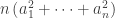 is on the right side of the inequality we wish to prove, and the expression
  is on the right side of the Schwarz inequality, this suggests that we should choose
  , or
, or  .
. is the square of the expression on the right side of the Schwarz inequality, this suggests that we should choose
  is the square of the expression
  on the left side of the Schwarz inequality, so that
  . Since
  this suggests that we choose
  .
. . If
. If  as noted earlier. Whether
  is positive or negative squaring it produces the same result, so that
  on the left hand side of the inequality.
 so that we have
  on the right hand side of the inequality.
 for any positive
  then
then  and
and 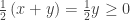 as long as
  . So
. So  and
and  . Combined with the previous result this shows that
  and
and  . We then have
  or
or  . This is the middle step of the one-line proof of the Schwarz inequality shown above.
 for any
  . Substituting into the inequality we have
  or
or  . Adding
  to both sides of the inequality we have
  or
or 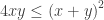 . If
. If  and we can take the square root of both sides of the inequality to obtain
  or
or  is a vector in
  then what is the angle
  that projects vectors in
  coordinate axis and the unit vector
  lying along that axis, whose
  . We have
  and
and  so that
  . We also have
  since the
  so that
  .
.

 or
or  then
then  and either
  or
or  so that
  . So in this case it is trivially true that
 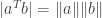 .) We first show that if
  . (We can do the division because per our assumption above both
 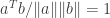 and if it is negative then we have
  . But
. But  where
where  or
or  .
. (or more generally,
  for some integer
  ), and
  (or more generally,
  for some integer
  so that
  . If
. If  . We then have
  so that
  . Combining the two equations we have
 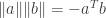 and the value
  that is closest to the point
  . Also find the point on the line through
  of
of  .
.

 with
with  being the multiple of
  of
of  .
.

 or
or
 is the point on the line through
  and thus of
  (where
  (where
 ![\|p\|^2 = \left[\left(a^Tb/a^Ta\right)a\right]^T \left[\left(a^Tb/a^Ta\right)a\right]](https://s0.wp.com/latex.php?latex=%5C%7Cp%5C%7C%5E2+%3D+%5Cleft%5B%5Cleft%28a%5ETb%2Fa%5ETa%5Cright%29a%5Cright%5D%5ET+%5Cleft%5B%5Cleft%28a%5ETb%2Fa%5ETa%5Cright%29a%5Cright%5D&bg=ffffff&fg=333333&s=0&c=20201002)
 is a scalar quantity we can bring it out of the transpose expression and then bring it to the left of the expression:

 at the right, so we can further simplify this expression as follows:


 is guaranteed to be positive but
  is not).

 be vectors in
  ,
,  and
and  where all
  ,
,  and
and  are real numbers.


 and the subspace
  of
of  , the orthogonal complement of
  where
where
 its orthogonal complement
  (the first and only row of

