
Exercise 2.2.9. Consider the following 


For what values of 


Answer: We perform elimination by subtracting 2 times the first row from the third row:

This completes elimination and produces the system 

Since the pivots of 


To find the general solution to 


From the second equation we must have 


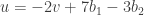
By setting 


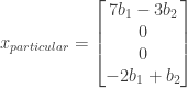
We can obtain a particular solution to
From the second equation we have 

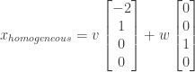
The general solution to

NOTE: This continues a series of posts containing worked out exercises from the (out of print) book Linear Algebra and Its Applications, Third Edition by Gilbert Strang.
If you find these posts useful I encourage you to also check out the more current Linear Algebra and Its Applications, Fourth Edition, Dr Strang’s introductory textbook Introduction to Linear Algebra, Fourth Edition
and the accompanying free online course, and Dr Strang’s other books
.

