Linear Algebra and Its Applications, Exercise 2.5.2

Exercise 2.5.2. Given the incidence matrix $A$ from exercise 2.5.1 and any vector $b$ in the column space of $A$ show that $b_1 + b_2 - b_3 = 0$ . Prove the same result based on the rows of $A$ . What is the implication for the potential differences around a loop?

Answer: From exercise 2.5.1 we have the incidence matrix

$A = \begin{bmatrix} 1&-1&0 \\ 0&1&-1 \\ 1&0&-1 \end{bmatrix}$

If $b = (b_1, b_2, b_3)$ is in the column space of $A$ then we have

$\begin{bmatrix} b_1 \\ b_2 \\ b_3 \end{bmatrix} = c_1 \begin{bmatrix} 1 \\ 0 \\ 1 \end{bmatrix} + c_2 \begin{bmatrix} -1 \\ 1 \\ 0 \end{bmatrix} + c_3 \begin{bmatrix} 0 \\ -1 \\ -1 \end{bmatrix}$

for some set of scalar coefficients $c_1$ , $c_2$ , and $c_3$ so that

$\begin{bmatrix} b_1 \\ b_2 \\ b_3 \end{bmatrix} = \begin{bmatrix} c_1 - c_2 \\ c_2 - c_3 \\ c_1 - c_3 \end{bmatrix}$

We then have

$b_1 + b_2 - b_3 = (c_1 - c_2) + (c_2 - c_3) - (c_1 - c_3)$

$= (c_1 - c_1) + (c_2 - c_2) + (c_3 - c_3) = 0 + 0 + 0 = 0$

We therefore have $b_1 + b_2 - b_3 = 0$ for all vectors $b$ in the column space of $A$ .

Turning to the rows of $A$ if $Ax = b$ we have

$\begin{bmatrix} 1&-1&0 \\ 0&1&-1 \\ 1&0&-1 \end{bmatrix} \begin{bmatrix} x_1 \\ x_2 \\ x_3 \end{bmatrix} = \begin{bmatrix} b_1 \\ b_2 \\ b_3 \end{bmatrix}$

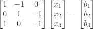
which corresponds to the system of equations

$\setlength\arraycolsep{0.2em}\begin{array}{rcrcrcr} x_1&-&x_2&&&=&b_1 \\ &&x_2&-&x_3&=&b_2 \\ x_1&&&-&x_3&=&b_3 \end{array}$

We then have

$b_1 + b_2 - b_3 = (x_1 - x_2) + (x_2 - x_3) - (x_1 - x_3)$

$= (x_1 - x_1) + (x_2 - x_2) + (x_3 - x_3) = 0 + 0 + 0 = 0$

We also have

$(x_1 - x_2) + (x_2 - x_3) - (x_1 - x_3)$

$= (x_1 - x_2) + (x_2 - x_3) + (x_3 - x_1)$

so that

$(x_1 - x_2) + (x_2 - x_3) + (x_3 - x_1) = 0$

The 3 by 3 incidence matrix $A$ represents a graph with three nodes and three edges and hence one loop. Each node of the graph is represented by a column of $A$ and each edge by a row of $A$ . The first row represents edge 1 from node 2 to node 1 (i.e., leaving node 2 and entering node 1). The second row represents edge 2 from node 3 to node 2. The third row represents edge 3 from node 3 to node 1.

If the vector $x$ represents potentials at the nodes ( $x_1$ at node 1, $x_2$ at node 2, and $x_3$ at node 3) then $x_1 - x_2$ is the potential difference along edge 1 (from node 2 to node 1), $x_2 - x_3$ is the potential difference along edge 2 (from node 3 to node 2) and $x_3 - x_1$ is the potential difference along edge 3 (from node 3 to node 1). From the equations above we see that the sum of the potential differences around the loop is zero (Kirchoff‘s Voltage Law).

NOTE: This continues a series of posts containing worked out exercises from the (out of print) book Linear Algebra and Its Applications, Third Edition by Gilbert Strang.

If you find these posts useful I encourage you to also check out the more current Linear Algebra and Its Applications, Fourth Edition, Dr Strang’s introductory textbook Introduction to Linear Algebra, Fourth Edition and the accompanying free online course, and Dr Strang’s other books.

Buy me a snack to sponsor more posts like this!

Linear Algebra and Its Applications, Exercise 2.5.2

Leave a Reply Cancel reply

Archives

Meta

Linear Algebra and Its Applications, Exercise 2.5.2

Share this:

Like this:

Related

Leave a Reply Cancel reply

Archives

Meta