Linear Algebra and Its Applications, Exercise 2.5.11

Exercise 2.5.11. Given the incidence matrix from exercise 2.5.10 with the final column removed and a diagonal matrix $C$ with elements 1, 2, 2, and 1, write the equations for the system

$\begin{array}{rcrcr} C^{-1}y&+&Ax&=&0 \\ A^Ty&&&=&f \end{array}$

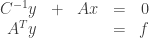
Show that eliminating $y$ gives the system $A^TCAx = -f$ and solve the system for $f = (1, 1, 6)$ . If $f = (1, 1, 6)$ represents the currents entering nodes 1, 2, and 3 of the graph, calculate the potentials at each node and the currents on each edge.

Answer: Removing the final column from the matrix in exercise 2.5.10 gives us the new matrix

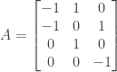
$A = \begin{bmatrix} -1&1&0 \\ -1&0&1 \\ 0&1&0 \\ 0&0&-1 \end{bmatrix}$

The diagonal matrix

$C = \begin{bmatrix} 1&0&0&0 \\ 0&2&0&0 \\ 0&0&2&0 \\ 0&0&0&1 \end{bmatrix}$

has as its inverse

$C^{-1} = \begin{bmatrix} 1&0&0&0 \\ 0&\frac{1}{2}&0&0 \\ 0&0&\frac{1}{2}&0 \\ 0&0&0&1 \end{bmatrix}$

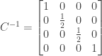
(Recall from Note 4 of section 1.6, “Inverses and Transposes”, that the inverse of a diagonal matrix $D$ with nonzero entries on the diagonal is itself a diagonal matrix, with the entries on the diagonal of $D^{-1}$ equal to the reciprocals of the corresponding entries on the diagonal of $D$ .)

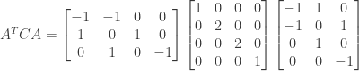
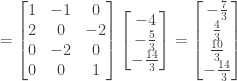
We can thus express the system $C^{-1}y + Ax = 0$ in matrix form as

$\begin{bmatrix} 1&0&0&0 \\ 0&\frac{1}{2}&0&0 \\ 0&0&\frac{1}{2}&0 \\ 0&0&0&1 \end{bmatrix} \begin{bmatrix} y_1 \\ y_2 \\ y_3 \\ y_4 \end{bmatrix} + \begin{bmatrix} -1&1&0 \\ -1&0&1 \\ 0&1&0 \\ 0&0&-1 \end{bmatrix} \begin{bmatrix} x_1 \\ x_2 \\ x_3 \end{bmatrix}$

$= \begin{bmatrix} y_1 \\ \frac{1}{2}y_2 \\ \frac{1}{2}y_3 \\ y_4 \end{bmatrix} + \begin{bmatrix} -x_1+x_2 \\ -x_1+x_3 \\ x_2 \\ -x_3 \end{bmatrix} = \begin{bmatrix} 0 \\ 0 \\ 0 \\ 0 \end{bmatrix}$

We can express the system $A^Ty = f$ in matrix form as

$\begin{bmatrix} -1&-1&0&0 \\ 1&0&1&0 \\ 0&1&0&-1 \end{bmatrix} \begin{bmatrix} y_1 \\ y_2 \\ y_3 \\ y_4 \end{bmatrix}$

$= \begin{bmatrix} -y_1-y_2 \\ y_1+y_3 \\ y_2-y_4 \end{bmatrix} = \begin{bmatrix} f_1 \\ f_2 \\ f_3 \end{bmatrix}$

This corresponds to the following system of equations:

$\begin{array}{rcrcrcrcrcrcrcr} y_1&&&&&&&-&x_1&+&x_2&&&=&0 \\ &&\frac{1}{2}y_2&&&&&-&x_1&&&+&x_3&=&0 \\ &&&&\frac{1}{2}y_3&&&&&+&x_2&&&=&0 \\ &&&&&&y_4&&&&&-&x_3&=&0 \\ -y_1&-&y_2&&&&&&&&&&&=&f_1 \\ y_1&&&+&y_3&&&&&&&&&=&f_2 \\ &&y_2&&&-&y_4&&&&&&&=&f_3 \end{array}$

Going back to the original two equations

$\begin{array}{rcrcr} C^{-1}y&+&Ax&=&0 \\ A^Ty&&&=&f \end{array}$

we can eliminate $y$ by multiplying the first equation by $A^TC$ to get $A^TCC^{-1}y + A^TCAx = 0$ or $A^Ty + A^TCAx = 0$ and then subtracting the second equation from this to get $A^TCAx = -f$ .

We have

$A^TCA = \begin{bmatrix} -1&-1&0&0 \\ 1&0&1&0 \\ 0&1&0&-1 \end{bmatrix} \begin{bmatrix} 1&0&0&0 \\ 0&2&0&0 \\ 0&0&2&0 \\ 0&0&0&1 \end{bmatrix} \begin{bmatrix} -1&1&0 \\ -1&0&1 \\ 0&1&0 \\ 0&0&-1 \end{bmatrix}$

$= \begin{bmatrix} -1&-2&0&0 \\ 1&0&2&0 \\ 0&2&0&-1 \end{bmatrix} \begin{bmatrix} -1&1&0 \\ -1&0&1 \\ 0&1&0 \\ 0&0&-1 \end{bmatrix} = \begin{bmatrix} 3&-1&-2 \\ -1&3&0 \\ -2&0&3 \end{bmatrix}$

If $f = (1, 1, 6)$ the system $A^TCAx = -f$ can therefore be expressed in matrix form as

$\begin{bmatrix} 3&-1&-2 \\ -1&3&0 \\ -2&0&3 \end{bmatrix} \begin{bmatrix} x_1 \\ x_2 \\ x_3 \end{bmatrix} = \begin{bmatrix} -1 \\ -1 \\ -6 \end{bmatrix}$

or as the system of equations

$\begin{array}{rcrcrcr} 3x_1&-&x_2&-&2x_3&=&-1 \\ -x_1&+&3x_2&&&=&-1 \\ -2x_1&&&+&3x_3&=&-6 \end{array}$

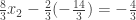
We begin elimination by multiplying the first equation by -1/3 and subtracting it from the second equation, and multiplying the first equation by -2/3 and subtracting it from the third equation. The result is the following system:

$\begin{array}{rcrcrcr} 3x_1&-&x_2&-&2x_3&=&-1 \\ &&\frac{8}{3}x_2&-&\frac{2}{3}x_3&=&-\frac{4}{3} \\ &&-\frac{2}{3}x_2&+&\frac{5}{3}x_3&=&-\frac{20}{3} \end{array}$

We then multiply the second equation by -1/4 and subtract it from the third equation:

$\begin{array}{rcrcrcr} 3x_1&-&x_2&-&2x_3&=&-1 \\ &&\frac{8}{3}x_2&-&\frac{2}{3}x_3&=&-\frac{4}{3} \\ &&&&\frac{3}{2}x_3&=&-7 \end{array}$

Solving for $x_3$ we have $x_3 = \frac{2}{3}(-7) = -\frac{14}{3}$ . Substituting the value of $x_3$ into the second equation we have $\frac{8}{3}x_2 - \frac{2}{3}(-\frac{14}{3}) = -\frac{4}{3}$ or $\frac{8}{3}x_2 = -\frac{4}{3} - \frac{28}{9} = -\frac{40}{9}$ so that $x_2 = \frac{3}{8}(-\frac{40}{9}) = -\frac{5}{3}$ . Finally we substitute the values of $x_2$ and $x_3$ into the first equation to obtain $3x_1 -(-\frac{5}{3})-2(-\frac{14}{3}) = -1$ or $3x_1 + 11 = -1$ so that $x_1 = \frac{1}{3}(-12) = -4$ .

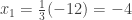
The solution to the system $A^TCAx = -f$ when $f = (1, 1, 6)$ is thus $x = (-4, -\frac{5}{3}, -\frac{14}{3})$ . If $f = (1, 1, 6)$ represents the currents into each of nodes 1, 2, and 3 respectively then $x = (-4, -\frac{5}{3}, -\frac{14}{3})$ represents the potentials at each of those nodes.

What are the currents along the edges? To determine that we must solve for $y$ . Since $C^{-1}y + Ax = 0$ we have $y = -CAx$ or

$y = \begin{bmatrix} -1&0&0&0 \\ 0&-2&0&0 \\ 0&0&-2&0 \\ 0&0&0&-1 \end{bmatrix} \begin{bmatrix} -1&1&0 \\ -1&0&1 \\ 0&1&0 \\ 0&0&-1 \end{bmatrix} \begin{bmatrix} -4 \\ -\frac{5}{3} \\ -\frac{14}{3} \end{bmatrix}$

$= \begin{bmatrix} 1&-1&0 \\ 2&0&-2 \\ 0&-2&0 \\ 0&0&1 \end{bmatrix} \begin{bmatrix} -4 \\ -\frac{5}{3} \\ -\frac{14}{3} \end{bmatrix} = \begin{bmatrix} -\frac{7}{3} \\ \frac{4}{3} \\ \frac{10}{3} \\ -\frac{14}{3} \end{bmatrix}$

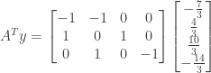
We can check this answer using the equation $A^Ty = f$

$A^Ty = \begin{bmatrix} -1&-1&0&0 \\ 1&0&1&0 \\ 0&1&0&-1 \end{bmatrix} \begin{bmatrix} -\frac{7}{3} \\ \frac{4}{3} \\ \frac{10}{3} \\ -\frac{14}{3} \end{bmatrix}$

$= \begin{bmatrix} \frac{3}{3} \\ \frac{3}{3} \\ \frac{18}{3} \end{bmatrix} = \begin{bmatrix} 1 \\ 1 \\ 6 \end{bmatrix} = f$

So $y = (-\frac{7}{3}, \frac{4}{3}, \frac{10}{3}, -\frac{14}{3})$ represents the currents flowing along edges 1, 2, 3, and 4 respectively.

NOTE: This continues a series of posts containing worked out exercises from the (out of print) book Linear Algebra and Its Applications, Third Edition by Gilbert Strang.

If you find these posts useful I encourage you to also check out the more current Linear Algebra and Its Applications, Fourth Edition, Dr Strang’s introductory textbook Introduction to Linear Algebra, Fourth Edition and the accompanying free online course, and Dr Strang’s other books.

Buy me a snack to sponsor more posts like this!

Linear Algebra and Its Applications, Exercise 2.5.11

Leave a Reply Cancel reply

Archives

Meta

Linear Algebra and Its Applications, Exercise 2.5.11

Share this:

Like this:

Related

Leave a Reply Cancel reply

Archives

Meta