Linear Algebra and Its Applications, Exercise 2.5.16

Exercise 2.5.16. Suppose we have a directed graph with four nodes and five edges as follows:

edge 1 from node 1 to node 2
edge 2 from node 2 to node 3
edge 3 from node 1 to node 3
edge 4 from node 1 to node 4
edge 5 from node 3 to node 4

Also assume that the graph is grounded at node 4. Do the following:

Describe the current laws $A^Ty = 0$ at the three ungrounded nodes 1, 2, and 3.
Describe how the current law at the grounded node 4 follows from the current laws at the other three nodes.
Specify the rank of $A^T$ .
Relate the solutions to $A^Ty = 0$ to the loops in the graph.

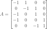
Answer: We start by constructing the incidence matrix for the network; it contains 5 rows corresponding to the edges and 4 columns corresponding to the nodes:

$A = \begin{bmatrix} -1&1&0&0 \\ 0&-1&1&0 \\ -1&0&1&0 \\ -1&0&0&1 \\ 0&0&-1&1\end{bmatrix}$

The system $A^Ty = 0$ can be expressed in matrix form as

$\begin{bmatrix} -1&0&-1&-1&0 \\ 1&-1&0&0&0 \\ 0&1&1&0&-1 \\ 0&0&0&1&1 \end{bmatrix} \begin{bmatrix} y_1 \\ y_2 \\ y_3 \\ y_4 \\ y_5 \end{bmatrix} = \begin{bmatrix} 0 \\ 0 \\ 0 \\ 0 \end{bmatrix}$

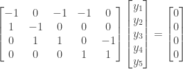
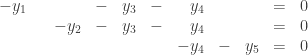
a) The equations corresponding to the current laws for the first three (ungrounded) nodes are

$\begin{array}{rcrcrcrcrcrcr} -y_1&&&-&y_3&-&y_4&&&=&0 \\ y_1&-&y_2&&&&&&&=&0 \\ &&y_2&+&y_3&&&-&y_5&=&0 \end{array}$

b) The equation for the current law at the grounded node is $y_4+y_5=0$ . It can be derived from the three equations above by adding the first equation to the second equation to produce the equation $-y_2-y_3-y_4 = 0$ and then adding this equation to the third equation to produce $-y_4-y_5=0$ or $y_4+y_5=0$ .

c) From inspection $A^T$ appears to have three pivots (in columns 1, 2, and 4) and therefore has rank 3. We can confirm this via elimination:

$\begin{bmatrix} -1&0&-1&-1&0 \\ 1&-1&0&0&0 \\ 0&1&1&0&-1 \\ 0&0&0&1&1 \end{bmatrix} \Rightarrow \begin{bmatrix} -1&0&-1&-1&0 \\ 0&-1&-1&-1&0 \\ 0&1&1&0&-1 \\ 0&0&0&1&1 \end{bmatrix}$

$\Rightarrow \begin{bmatrix} -1&0&-1&-1&0 \\ 0&-1&-1&-1&0 \\ 0&0&0&-1&-1 \\ 0&0&0&1&1 \end{bmatrix} \Rightarrow \begin{bmatrix} -1&0&-1&-1&0 \\ 0&-1&-1&-1&0 \\ 0&0&0&-1&-1 \\ 0&0&0&0&0 \end{bmatrix}$

As noted above, there are three pivots in columns 1, 2, and 4, and thus the rank of $A^T$ is 3.

d) From the elimination above we see that $y_1$ , $y_2$ , and $y_4$ are basic variables and $y_3$ and $y_5$ are free variables. The resulting echelon matrix corresponds to the following system of equations:

$\begin{array}{rcrcrcrcrcrcr} -y_1&&&-&y_3&-&y_4&&&=&0 \\ &&-y_2&-&y_3&-&y_4&&&=&0 \\ &&&&&&-y_4&-&y_5&=&0 \end{array}$

If we set $y_3 =1$ and $y_5 = 0$ then from the third equation we have $y_4 = 0$ . Substituting into the second equation we have $y_2 = -1$ . Substituting into the first equation we have $y_1 = -1$ .

If we set $y_3 =0$ and $y_5 = 1$ then from the third equation we have $y_4 = -1$ . Substituting into the second equation we have $y_2 = 1$ . Substituting into the first equation we have $y_1 = 1$ .

The general solution to $A^Ty = 0$ is thus given by

$y_3 \begin{bmatrix} -1 \\ -1 \\ 1 \\ 0 \\ 0 \end{bmatrix} + y_5 \begin{bmatrix} 1 \\ 1 \\ 0 \\ -1 \\ 1 \end{bmatrix}$

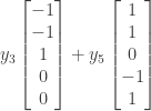
The first term can be interpreted as a set of currents around the upper loop in the graph: In the bottom edge we have a current of $y_3$ from node 1 to node 3. We then have a current of $-y_3$ from node 2 to node 3, equivalent to a current of $y_3$ from node 3 to node 2. Finally we have a current of $-y_3$ from node 1 to node 2, equivalent to a current of $y_3$ from node 2 to node 1. The net current around the loop is zero.

The second term can be interpreted as a set of currents around the outer loop in the graph: In the top left edge we have a current of $y_5$ from node 1 to node 2. We then have a current of $y_5$ from node 2 to node 3 along the upper right edge, and a current of $y_5$ from node 3 to node 4 along the bottom right edge. Finally we have a current of $-y_5$ from node 1 to node 4, equivalent to a current of $y_5$ from node 4 to node 1. Again the net current around the loop is zero.

NOTE: This continues a series of posts containing worked out exercises from the (out of print) book Linear Algebra and Its Applications, Third Edition by Gilbert Strang.

If you find these posts useful I encourage you to also check out the more current Linear Algebra and Its Applications, Fourth Edition, Dr Strang’s introductory textbook Introduction to Linear Algebra, Fourth Edition and the accompanying free online course, and Dr Strang’s other books.

Buy me a snack to sponsor more posts like this!

Linear Algebra and Its Applications, Exercise 2.5.16

Leave a Reply Cancel reply

Archives

Meta

Linear Algebra and Its Applications, Exercise 2.5.16

Share this:

Like this:

Related

Leave a Reply Cancel reply

Archives

Meta