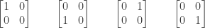
Exercise 2.6.16. Consider the space of 2 by 2 matrices. Any such matrix can be represented as the linear combination of the matrices

that serve as a basis for the space. Find a matrix corresponding to the linear transformation of transposing 2 by 2 matrices, and explain why .

Answer: Each of the elementary 2 by 2 matrices can be considered as equivalent to one of the elementary vectors in

(Simply read off the entries in the 2 by 2 matrices starting with the first row left to right and then the second row left to right.)

We want to transpose each of the elementary 2 by 2 matrices into the following matrices:

corresponding to the following vectors in

In other words we must have , , , and .

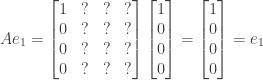
Since when multiplying the first row of by the entries of (which produces the first entry in the resulting vector) we must produce 1, and when multiplying the second through fourth row of by the entries of we must produce 0. This means must look as follows:

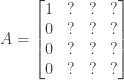
Note that we don’t care what the other entries in are, since when multiplying those entries will end up multiplying zeroes:

Since when multiplying the first row of by the entries of we must produce 0,  and similarly when multiplying the second and fourth rows of by the entries of . However when multiplying the third row of by the entries of (which produces the third entry in the resulting vector) we must produce 1. This means must look as follows:

Note again that we don’t care what the other entries in are, since when multiplying those entries will end up multiplying zeroes:

We next have so when multiplying the second row of by the entries of we must produce 1,  and when multiplying the other rows of by the entries of must produce 0. This means must look as follows:

so that

Finally since when multiplying the first, second, and third rows of by the entries of we must produce 0, and when multiplying the fourth row of by the entries of we must produce 1. This means must look as follows:

with

Combining the above results we see that

Note that we could have achieved the same result by having each column of be the vector into which the corresponding elementary vector should be transformed. In other words, the first column of should be (since transforms into ), the second column should be (since transforms into ), and similarly the third and fourth columns should be and respectively.

When multiplying by itself we see that

In other words, applying twice to a given vector leaves that vector unchanged. This effect can be explained in multiple ways.

First, when applied to vectors in the matrix permutes the second and third entries of the vectors but leaves the first and fourth entries unchanged:

Applying again reverses the effect of the permutation of the second and third entries, again leaving the first and fourth entries unchanged, and thus restores the original vector.

Second, when applied to our original space of 2 by 2 matrices has the effect of transposing a matrix, transforming

into

Applying twice has the effect of taking the transpose of the transpose. Since for any matrix this has the effect of restoring the original 2 by 2 matrix.

NOTE: This continues a series of posts containing worked out exercises from the (out of print) book Linear Algebra and Its Applications, Third Edition by Gilbert Strang.

If you find these posts useful I encourage you to also check out the more current Linear Algebra and Its Applications, Fourth Edition, Dr Strang’s introductory textbook Introduction to Linear Algebra, Fourth Edition and the accompanying free online course, and Dr Strang’s other books.

 Buy me a snack to sponsor more posts like this!