Review exercise 2.6. Given the matrices

find bases for each of their four fundamental subspaces.
Answer: The second column of  is equal to twice the first column so the rank of (and the dimension of the column space of ) is 1. The first column
  is a basis for the column space of .
The dimension of the row space of is also 1 (the rank of ), and the first row  is a basis for the row space of .
We can reduce to echelon form by subtracting 3 times the first row from the second row:

The resulting echelon matrix has one pivot, with  a basic variable and
  a free variable. Setting
  we have from the first row of the echelon matrix
  or
or  . The vector
  is thus a basis for the nullspace of .
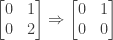
The left nullspace of is the nullspace of

We can reduce  to echelon form by subtracting 2 times the first row from the second row:

The resulting echelon matrix has one pivot, with a basic variable and a free variable. Setting we have from the first row of the echelon matrix  or
or  . The vector
  is thus a basis for the nullspace of and for the left nullspace of .
As with , the second column of  is equal to twice the first column, so the rank of (and the dimension of the column space of ) is 1. The first column
  is a basis for the column space of .
The dimension of the row space of (the rank of ) is also 1, and the second row is a basis for the row space of . Note that this is the same as the basis for the row space of so that the row spaces of and are identical.
We can transform the matrix to echelon form simply by exchanging the first and second rows:

The resulting echelon matrix has one pivot, with a basic variable and a free variable. Setting we have from the first row of the echelon matrix or . The vector is thus a basis for the nullspace of . This is the same as the basis for the nullspace of so that the nullspaces of and are identical, like the row spaces.
The left nullspace of is the nullspace of

We can reduce  to echelon form by subtracting 2 times the first row from the second row:
The resulting echelon matrix has one pivot, with a basic variable and a free variable. Setting  we have from the first row of the echelon matrix
  . The vector
  is thus a basis for the nullspace of and for the left nullspace of .
The matrix  is already in echelon form, with pivots in the first and second columns. It has rank 2 and the first and second columns and
  respectively form a basis for the column space. Note that since the second column is equal to the first column plus the fourth column, an alternate basis for the column space consists of the first and fourth columns and respectively.
The dimension of the row space of (the rank of ) is also 2, and the two rows  and
and  of are a basis for the row space of .
In the system  we have and as basic variables and
  and
and  as free variables. If we set
  and
and  then from the second row of we have
  or . From the first row of we then have
  or
or  . Thus one solution to is
  .
.
If we set  and
and  then from the second row of we have
  or
or  . From the first row of we then have
  or . Thus a second solution to is
  . The two solutions and are a basis for the nullspace of .
Finally, since has rank  and has
  rows, the dimension of the left nullspace is
  . This means that the only vector in the left nullspace is the zero vector
  .
.
NOTE: This continues a series of posts containing worked out exercises from the (out of print) book Linear Algebra and Its Applications, Third Edition by Gilbert Strang.
If you find these posts useful I encourage you to also check out the more current Linear Algebra and Its Applications, Fourth Edition , Dr Strang’s introductory textbook Introduction to Linear Algebra, Fourth Edition
 and the accompanying free online course, and Dr Strang’s other books
 .
.
 Buy me a snack to sponsor more posts like this!


