Exercise 3.1.7. For the matrix
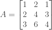
find vectors  and
and  such that is orthogonal to the row space of
  and is orthogonal to the column space of >
Answer: The nullspace of is orthogonal to the row space of . We can therefore find a suitable vector by solving the system  .
.
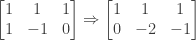
To solve the system we perform Gaussian elimination. We start by subtracting 2 times row 1 from row 2:

and then subtract 3 times row 1 from row 3:

Finally we subtract row 2 from row 3:
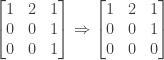
The echelon matrix has 2 pivots in columns 1 and 3, so  and
and  are basic variables and
  is a free variable.
Setting  from row 2 we have
  and from row 1 we have
  or
or  . So the vector
  is a solution to the system, a basis for the nullspace of , and a vector orthogonal to the row space of .
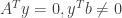
The left nullspace of is orthogonal to the column space of . We can therefore find a suitable vector by solving the system  .
.
To solve the system we perform Gaussian elimination. We start by subtracting 2 times row 1 from row 2:

and then subtract 1 times row 1 from row 3:
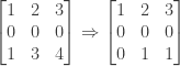
Finally we exchange rows 2 and row 3:

The resulting echelon matrix has 2 pivots in columns 1 and 2, so  and
and  are basic variables and
  is a free variable.
Setting  from row 2 we have
  or
or  . From row 1 we have
  or
or  . So the vector
  is a solution to the system, a basis for the left nullspace of , and a vector orthogonal to the column space of .
NOTE: This continues a series of posts containing worked out exercises from the (out of print) book Linear Algebra and Its Applications, Third Edition by Gilbert Strang.
If you find these posts useful I encourage you to also check out the more current Linear Algebra and Its Applications, Fourth Edition , Dr Strang’s introductory textbook Introduction to Linear Algebra, Fourth Edition
 and the accompanying free online course, and Dr Strang’s other books
 .
.
 Buy me a snack to sponsor more posts like this!


 and
and  find a homogeneous system in three unknowns whose solutions are the linear combinations of the vectors.
 . This means that for any vector
 for all vectors
 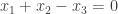 .)
.) spanned by the vectors

 , from the second row we have
  or
or  . From the first row we have
  or
or  .
. and
and  are orthogonal subspaces. Show that their intersection consists only of the zero vector.
 for any vectors
  in
in  in
in  . But this means that
  and thus that
  .
. .
. and
and  in
in  is a vector orthogonal to both
 or
or  . From row 1 we have
  or
or  . So the vector
  is a solution to the system and thus a vector orthogonal to
 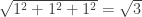 , the length of
  , and the length of


 and
and  are orthogonal to
  but not to each other.
 is an invertible matrix, describe why row
  of
of  of
of  are orthogonal in the case
  .
. . The identity matrix
  has ones on the diagonal (i.e., when
  ) and zeros otherwise (when
  entry of the matrix product
  is equal to the inner product of row
  and
and  being orthogonal.
 and the line through the origin and
  . If the two lines are perpendicular we have
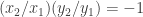
 we have

 give an example of linearly independent vectors that are not mutually orthogonal, as well as mutually orthogonal vectors that are not linearly independent.
 and
and  are linearly independent, since the second vector cannot be expressed as a scalar times the first vector. However the two vectors are not orthogonal since their inner product is
  .
. is orthogonal to every vector in
