Review exercise 2.20. Consider the set of all 5 by 5 permutation matrices. How many such matrices are there? Are the matrices linearly independent? Do the matrices span the set of all 5 by 5 matrices?
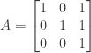
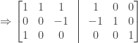
Answer: An example member of this set is

Note that for any such permutation matrix each row has the value 1 in one column and the value 0 in all other columns. Also note that if a given row has a 1 in a given column then no other row can have a 1 in that column.
This allows us to calculate the number of permutation matrices as follows: For the first row we have five columns in which to put a 1. Having chosen a 1 column for the first row, we then have four choices for the column to contain a 1 in the second row (because we can’t put it in the same column as in the first row). Having chosen the 1 columns for the first two rows we have three choices for the 1 column in the third row, and having chosen the 1 columns for the first three rows we have two choices for the 1 column in the fourth row. Finally, having chosen the 1 columns for the first four rows there is only one choice for the 1 column in the fifth row.
The number of 5 by 5 permutation matrices is therefore

(In general the number of  by permutation matrices is
  .)
.)
The set of 5 by 5 matrices has dimension  . Since the number of 5 by 5 permutation matrices is greater than 25 the set of permutation matrices cannot be linearly independent.
Does the set of 5 by 5 permutation matrices span the space of all 5 by 5 matrices? One way to address this question is to first look at the set of 3 by 3 permutation matrices, of which there are  matrices. A linear combination of such matrices looks as follows:
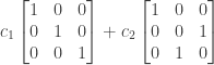


Notice that for each row in the resulting matrix the sum of the entries in the row is the same, namely  .
.
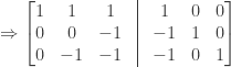
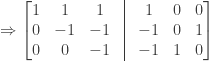
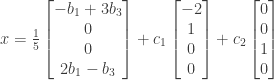
Now consider the set of 5 by 5 permutation matrices  and consider forming a linear combination of those matrices; this produces a matrix


for some arbitrary set of scalars  .
.
Consider an arbitrary row of  . Of the 120 5 by 5 permutation matrices there are 24 permutation matrices that have the value 1 in column 1, so the entry for column 1 in that row of will be the sum of the 24 scalars that multiply those matrices. Similarly, there is a different set of 24 permutation matrices that have a 1 in column 2, so the entry for column 2 in that row of will be the sum of the different 24 scalars that multiply those matrices. Continuing in this way for columns 3 through 5, we see that each scalar contributes to the value of one and only one column in that row of , and that (as in the 3 by 3 case) the sum of the entries for all columns in that row is equal to the sum of the 120 scalars, or
  .
.
We chose an arbitrary row, so this same argument applies to all rows of : the sum of the entries for all columns in each row of is equal to the same value .
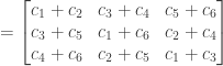
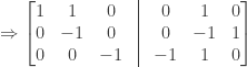
There are matrices for which the sum of the entries in each row is not equal, for example the matrix

for which the sum of the entries in the first row is 2 and the sum of the entries in all other rows is 1. The matrix  cannot be expressed as a linear combination of the 5 by 5 permutation matrices (otherwise the sum of the entries in each row of would be the same), and thus the set of 5 by 5 permutation matrices does not span the space of all 5 by 5 matrices.
NOTE: This continues a series of posts containing worked out exercises from the (out of print) book Linear Algebra and Its Applications, Third Edition by Gilbert Strang.
If you find these posts useful I encourage you to also check out the more current Linear Algebra and Its Applications, Fourth Edition , Dr Strang’s introductory textbook Introduction to Linear Algebra, Fourth Edition
 and the accompanying free online course, and Dr Strang’s other books
 .
.
 Buy me a snack to sponsor more posts like this!


![[T]](https://s0.wp.com/latex.php?latex=%5BT%5D&bg=ffffff&fg=333333&s=0&c=20201002)
![[T]^{-1}](https://s0.wp.com/latex.php?latex=%5BT%5D%5E%7B-1%7D&bg=ffffff&fg=333333&s=0&c=20201002)
![[T] = \begin{bmatrix} 1&1&1 \\ 1&1&0 \\ 1&0&0 \end{bmatrix}](https://s0.wp.com/latex.php?latex=%5BT%5D+%3D+%5Cbegin%7Bbmatrix%7D+1%261%261+%5C%5C+1%261%260+%5C%5C+1%260%260+%5Cend%7Bbmatrix%7D&bg=ffffff&fg=333333&s=0&c=20201002)


![[T]^{-1} = \begin{bmatrix} 0&0&1 \\ 0&1&-1 \\ 1&-1&0 \end{bmatrix}](https://s0.wp.com/latex.php?latex=%5BT%5D%5E%7B-1%7D+%3D+%5Cbegin%7Bbmatrix%7D+0%260%261+%5C%5C+0%261%26-1+%5C%5C+1%26-1%260+%5Cend%7Bbmatrix%7D&bg=ffffff&fg=333333&s=0&c=20201002)

![[T][T]^{-1} = \begin{bmatrix} 1&1&1 \\ 1&1&0 \\ 1&0&0 \end{bmatrix} \begin{bmatrix} 0&0&1 \\ 0&1&-1 \\ 1&-1&0 \end{bmatrix}](https://s0.wp.com/latex.php?latex=%5BT%5D%5BT%5D%5E%7B-1%7D+%3D+%5Cbegin%7Bbmatrix%7D+1%261%261+%5C%5C+1%261%260+%5C%5C+1%260%260+%5Cend%7Bbmatrix%7D+%5Cbegin%7Bbmatrix%7D+0%260%261+%5C%5C+0%261%26-1+%5C%5C+1%26-1%260+%5Cend%7Bbmatrix%7D&bg=ffffff&fg=333333&s=0&c=20201002)

 ,
,  , and
, and  in its column space. Does
  , the number of rows of
  . However it does not have a left inverse
  is less than the number of columns
  .
. ,
,  , and
, and  in
in  ,
,  , and
, and  then we have


 satisfy in order for
  to have a solution?
 ?
?

 .
. corresponds to

 and
and  as basic variables and
  and
and  as basic variables. (Note that this would be true whether or not we do a row exchange to put the matrix in true echelon form.)
 . Setting
  and
and  , from the first equation we have
  or
or  . Setting
  and
and  , from the first equation we have
  or
or  .
.

 . From the first equation we have
  and from the third equation we have
  . Subtracting twice the first equation from the third equation we obtain
  or
or  .
.

 .
.
 and
and  are arbitrary scalars.
 if
if  is even and
  if
if  and the second row has the form
  . Every other odd row is equal to the first row: If
  is odd then
  is even, and
  for all odd
  .
. is even, and
  for all even
  with ones on the diagonal and at most one nonzero entry below the diagonal. What subspace is spanned by these matrices?
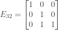
 then
then  .
. exists. We then have
 then
then  is a vector in
  and that
  for all
  . Show that
  and
and  we have
 for each of the elementary vectors
  . By the definition of the elementary vectors we have
  if
if  and
and  otherwise.
 we have
 for all
  .
. of
of  , and the number of columns
 ,
,  , and
, and  (since the two columns are linearly independent). Per box 2Q on page 96, since
  we are not guaranteed that a solution exists. So
 ,
,  , and
, and  we know that there is at least one solution to
  we know that there is more than one solution.
 we know that there may not be a solution to
  we know that there if there is a solution then it is not guaranteed to be unique.