
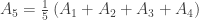
Review exercise 2.15. For each of the following, find a matrix 
i) there is either no solution or one solution to 
ii) there are an infinite number of solutions to 
iii) there is either no solution or an infinite number of solutions to
iv) there is exactly one solution for
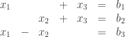
Answer: i) The following system of two equations in two unknowns

obviously has a solution no matter the value of 

then the resulting system may or may not have a solution depending on the value of 

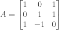
The system above corresponds to

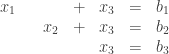
ii) In order for a system to have an infinite number of solutions we can specify more unknowns than there are equations, so that some variables are free variables that can take on any value. For example, if we start again with the system of two equations in two unknowns
we can add another unknown to obtain the following system of two equations in three unknowns:

This system has the general solution 

The system above corresponds to

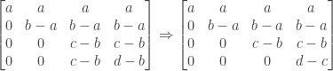
iii) The system of two equations in three unknowns in (ii) above has an infinite number of solutions. To allow for the possibility of having either an infinite number of solutions or no solution at all, we can follow the example of (i) above and add a third equation which might or might not be satisfiable depending on the value of 
For example, consider the following system of equations:
From (ii) above we know that 

So the system has an infinite number of solutions if 
The system above corresponds to
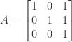
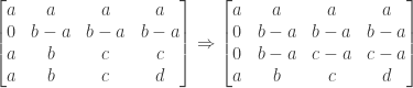
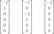
iv) Consider taking the system of three equations in three unknowns from (iii) above and changing the third equation as follows:
From the third equation we have 


This corresponds to
NOTE: This continues a series of posts containing worked out exercises from the (out of print) book Linear Algebra and Its Applications, Third Edition by Gilbert Strang.
If you find these posts useful I encourage you to also check out the more current Linear Algebra and Its Applications, Fourth Edition, Dr Strang’s introductory textbook Introduction to Linear Algebra, Fourth Edition
and the accompanying free online course, and Dr Strang’s other books
.
 ,
,  , and
, and  form a basis for the vector space
  ?
?


 . This means that the three columns are not linearly independent and thus the original three vectors cannot be a basis for
 and describe the conditions under which the columns of


 and thus the columns of
  ,
,  ,
,  , and
, and  .
. and
and  so that

 by
by  and has rank
  . What is the dimension of its nullspace?
 is the number of columns of
  .
.
 .
. ,
,  , and
, and  are basic variables and
  ,
,  , and
, and  are free variables.
 and
and  then from the third row of
  . From the second row of
  or
or  . Finally, from the first row of
  or
or  . So one solution to
  is
is  .
. and
and  . From the third row of
  or
or  . Finally, from the first row of
  or
or  . So a second solution to
  .
. and
and  . From the third row of
  or
or  .
.


 ,
,  , and
, and  are nonzero.
 . In particular the value multiplying the third row prior to subtracting from the fourth row is
  .
. to
to  be linear transformations from
 ![[A]](https://s0.wp.com/latex.php?latex=%5BA%5D&bg=ffffff&fg=333333&s=0&c=20201002) and
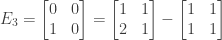
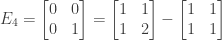
and ![[B]](https://s0.wp.com/latex.php?latex=%5BB%5D&bg=ffffff&fg=333333&s=0&c=20201002) be the
be the  to be the linear transformation represented by the matrix
 ![c[A]](https://s0.wp.com/latex.php?latex=c%5BA%5D&bg=ffffff&fg=333333&s=0&c=20201002) and define the vector sum
and define the vector sum  to be the linear transformation represented by the matrix
 ![[A]+[B]](https://s0.wp.com/latex.php?latex=%5BA%5D%2B%5BB%5D&bg=ffffff&fg=333333&s=0&c=20201002) .
. .
. for all
  and
and  )?
)?

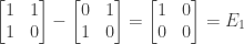
 equal to the identity matrix, i.e., leaving the order of rows unchanged.
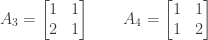
 are of the form:

 and
and  .
.

 through
  are of the form:


 through
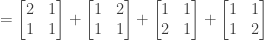
  are linearly dependent and that one of them can be expressed as a linear combination of the others.
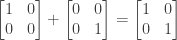
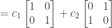
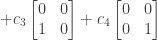
 we see that

 . Note that this implies that
  ; thus, for example the matrix
  and similarly for
  through
  spans
spans  positive vectors, analogous to
 through


 .
. .
. and row space spanned by
  .
. and a second arbitrary set of three vectors in
  determine whether a 6 by 5 matrix exists for which the first three vectors span the column space and the second three vectors span the row space.

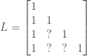
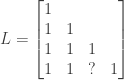
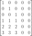
 . An easy way to find a matrix


 so that the second and third rows are multiples of the first row, and the second column is a multiple of the first column:


 and
and  as basic variables, and
  as a free variable. Setting
  or
or  . From the first row we then have
  or
or  . So
. So  is a solution for the homogeneous system, as is any multiple of that vector.
 and go back to the original system. From the second equation we have
  or
or  . From the first equation we have
  or
or  . So
. So  is a particular solution.
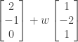

 is a basis for the column space of
  is a basis for the row space of
 or
or  is thus a basis for the nullspace of
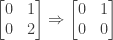
 to echelon form by subtracting 2 times the first row from the second row:
 or
or  . The vector
  is thus a basis for the nullspace of
  is a basis for the column space of

 we have from the first row of the echelon matrix
  . The vector
  is thus a basis for the nullspace of
  respectively form a basis for the column space. Note that since the second column is equal to the first column plus the fourth column, an alternate basis for the column space consists of the first and fourth columns
  and
and  of
of  we have
  and
and  then from the second row of
  or
or  or
or  . Thus one solution to
  .
. or
or  . From the first row of
  or
or  . The two solutions
  rows, the dimension of the left nullspace is
  . This means that the only vector in the left nullspace is the zero vector
  .
.
