Review exercise 2.3. State whether each of the following is true or false. If false, provide a counterexample.
i) If a subspace  is spanned by a set of
  vectors
  through
  then the dimension of is .
ii) If  and
and  are two subspaces of a vector space
  then the intersection of and is nonempty.
iii) For any matrix  if
if  then we have
  .
.
iv) For any matrix if is reduced to echelon form then the rows of the resulting matrix  form a unique basis for the row space of .
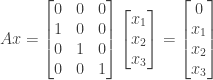
v) If is a square matrix and the columns of are linearly independent then the columns of  are also linearly independent.
Answer: i) The statement is false. The dimension of is the number of vectors in its basis, and the basis vectors have to be linearly independent. However it is possible that some of the vectors in the spanning set may be linear combinations of other vectors in the set; in that case would be larger than the number of basis vectors, and thus larger than the dimension of . For example, the vectors  ,
,  , and
, and  span
span  but the dimension of is 2, not 3.
ii) The statement is true. Every vector space contains the zero vector. Since and are subspaces they are also vector spaces in their own right, and therefore both contain the zero vector also. So the intersection of and is guaranteed to contain (at least) the zero vector and thus will always be nonempty.
iii) The statement is false. The matrix could be the zero matrix, in which case we would have  no matter what values
  and
and  had.
had.
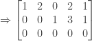
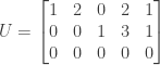
iv) The statement is false. The row space of is the same as the row space of (since the rows of are linear combinations of the rows of ) and the (nonzero) rows of do form a basis for . However this basis is not unique.
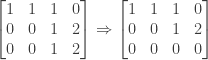
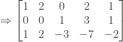
For example, suppose that

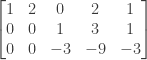
Then can be reduced to echelon form as

The vectors and  form a basis for the row space of but this basis is not unique. For example, the original rows and
  are also linearly independent and form a basis for the row space of .
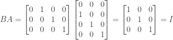
v) The statement is true. If the columns of are linearly independent then is nonsingular and has an inverse  . (See the discussion on page 98.) We then have

and also

So  is both a left and right inverse for and we see that is invertible with
 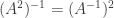 . But if is invertible then it is nonsingular and its columns are linearly independent.
UPDATE: Corrected a typo in the answer to (iv) (a reference to should have been a reference to ).
NOTE: This continues a series of posts containing worked out exercises from the (out of print) book Linear Algebra and Its Applications, Third Edition by Gilbert Strang.
If you find these posts useful I encourage you to also check out the more current Linear Algebra and Its Applications, Fourth Edition , Dr Strang’s introductory textbook Introduction to Linear Algebra, Fourth Edition
 and the accompanying free online course, and Dr Strang’s other books
 .
.
 Buy me a snack to sponsor more posts like this!


 . The rank of
  so the dimension of the nullspace of
  .
. so the dimension of the left nullspace of
  .
. ,
,  , or
, or  .
. . The coordinate vectors are not solutions to this equation and hence are not part of the nullspace.
 then we again have
  . The two vectors
  are thus basis vectors for the nullspace.
 and
and 
 ,
,  , and
, and 
 and
and  is in the subspace and can serve as a basis vector. If
  then we obtain a second basis vector
  and if
  and
and  .
.
 .
. are thus basis vectors for the subspace (which happens to be the nullspace of the matrix above).
 . So of the three vectors only two are linearly independent, and
  into
into  . What is the axis of rotation for the transformation? What is the angle of rotation?
 axes respectively.
 in the
  , which is also incorrect. We conclude that the axis of rotation must be somewhere between the
  in the
  that passes through the origin and the point
  , and is at an angle of 45 degrees from each of the axes and coordinate planes.
 in agreement with the argument above.
 , and applying it a third time sends
  from a vector space
  is invertible a) if for any
  in
in  and b) if
  implies that
  to
to 


![x = \sqrt[3]{b}](https://s0.wp.com/latex.php?latex=x+%3D+%5Csqrt%5B3%5D%7Bb%7D&bg=ffffff&fg=333333&s=0&c=20201002) exists and is a unique solution to
exists and is a unique solution to  . The transformation
  for all
  then there is no
  . The transformation
  exists and is a unique solution to
  . The transformation
  for all
  or
or  then there is no
  . Also note even for
  solutions to
  . The transformation
  and let
  . Show that
  is a member of
  for any scalar
  . By the
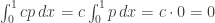
 is also a member of
  . By the


 is a constant.


 meeting this criterion. For the first basis vector we arbitrarily set
  and
and  . We then have

 corresponding to the polynomial
  .
. and
and  . We then have

 corresponding to the polynomial
  . Note that this vector is linearly independent of the first basis vector since it includes a term in
  that the first vector lacks.
 and
and  . We then have

 corresponding to the polynomial
  . Note that this vector is linearly independent of the first and second basis vectors since it includes a term in
  that those vectors lack.
 . But this is not the case.) The following vectors can thus serve as a basis for
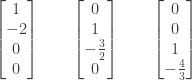
 ,
,  in
in 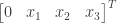 in
in  in
in  in
in  and
and  and what effects do they have?
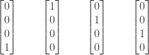
 through
  respectively will shift each of their entries to the right (or down, depending on your point of view) and produce the following vectors in


 respectively will shift each of their entries to the left (or up) and produce the following vectors in


 in
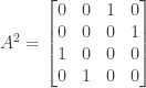
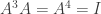
in  . Determine the effect of
  and explain why
  .
.
 ,
,  ,
,  , and
, and  .
. into
into 


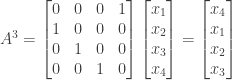
 we have


 and
and  . Since
