
Exercise 2.6.7. Describe the matrices representing the following transformations:
i) projecting all vectors onto the 

ii) reflecting all vectors through the
iii) rotating all vectors in the 
iv) rotating the
v) again carrying out the three rotations in succession, but through 180 degrees each time instead
Answer: i) The following matrix projects all vectors onto the

Note that this has the effect of multiplying the

ii) The following matrix reflects all vectors through the

Note that this has the effect of negating the

iii) In order to carry out this transformation, we start with the 2 by 2 matrix for rotation in the
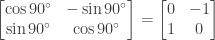
Moving to three dimensions, the following matrix rotates all vectors in the

Note that this has the effect of preserving the

iv) In order to carry out this transformation, we first use the matrix from the previous exercise that rotates all vectors in the
We then use the matrix that rotates all vectors in the

Note that this matrix is constucted by taking the 2 by 2 matrix for rotation by 90 degrees in the
Finally we use the matrix that rotates all vectors in the

We perform all three rotations by multiplying the matrices in reverse order:

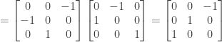
Note that this transformation is equivalent to rotating all vectors in the
v) In order to carry out this transformation, we start with the 2 by 2 matrix for rotation in the

Moving to three dimensions, we first use the matrix that rotates all vectors in the

We then use the matrix that rotates all vectors in the

Finally we use the matrix that rotates all vectors in the

We perform all three rotations by multiplying the matrices in reverse order:


Note that this transformation is equivalent to multiplying a vector by the identity matrix, leaving it unchanged.
UPDATE: Corrected the calculation of the cumulative effect of the three rotations in the answer to (iv). Thanks to Ji for pointing out my error.
NOTE: This continues a series of posts containing worked out exercises from the (out of print) book Linear Algebra and Its Applications, Third Edition by Gilbert Strang.
If you find these posts useful I encourage you to also check out the more current Linear Algebra and Its Applications, Fourth Edition, Dr Strang’s introductory textbook Introduction to Linear Algebra, Fourth Edition
and the accompanying free online course, and Dr Strang’s other books
.

 for which
  and thus leaves unchanged the entire
  ,
,  , and
, and  .
.


 transforms the
  is halfway between
  and
and  .
. . For example, if
  and
and  then
then


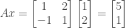
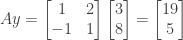


 into the vector
  . Consider also the circle formed by all points for which
  . What shape is the curve created by transforming all points on the circle by
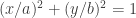
 and
and  . We know that for all points
  on the new curve we have
  and
and  . Since
  .
.

 and
and  . The new curve is thus an ellipse.
 through
  be the 8 rotation matrices and
  through
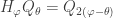
  the 5 reflection matrices. Note that the question is a bit ambiguous as to whether the reflections or rotations are done first; we assume that the reflections are done first, so that the product matrix


 is a rotation matrix formed by the product of
  ,
,  is a rotation matrix formed by the product of
  and
and  through
  are calculated similarly.
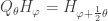
 is a rotation matrix formed by the product of
  and
and  is the rotation matrix formed by the product of
 is a reflection matrix formed by the product of
  is a reflection matrix formed by the product of
  and
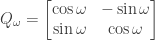
and  can be represented by the matrix
 (the
(the 


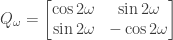
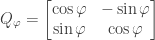
 that rotates vectors through an angle
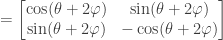
  that reflects vectors in the line through the origin with angle
  -line:

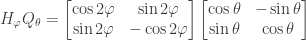
 in which we first reflect vectors in the line through the origin with angle


 -line.
 then this equation reduces to
  or
or  since
since  .
.
 . (Here we use the expression for a reflection matrix derived in the
  for some
  and then reflect it in the
  -line (the line for which
  ). The rotation takes
  to
to  and the reflection takes
  and then reflect it in the
  -line (the line for which
  ). The rotation takes
  and the reflection takes
  . The corresponding line of reflection is the
  -line (equivalent to the
  -line).
 and in the second case we would have
  . Subtracting 2 times the first equation from the second we have
 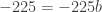 or
or  or
or  .
. . If this is the case then the matrix representing the reflection would be


 and in the second case we would have
  . Subtracting the first equation from the second we have
  or
or  . Substituting the value of
 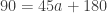 or
or  .
. . If this is the case then the matrix representing the rotation would be

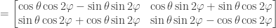
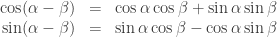
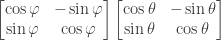
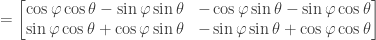
 the entries are expressed in terms of the sine and cosine of an expression containing
  and
and  . As a start toward proving that
  it might be useful to re-express
  and
and  in terms of the sine and cosine of

 and
and  .
.
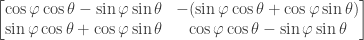
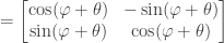
 we see that


 and
and  .)
.)


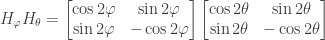
 so that the effect of applying a reflection through the
  .
. instead of through the angle
  . We therefore have
  except in the cases where
  or (more generally) the two angles differ by a multiple of
  . (The general case is because for any angle
  and likewise for the cosine.) In that case
  and the equivalent rotation matrix is
  corresponding to rotation through the zero angle.
 . If instead we take
  .
. . Let’s prove this conjecture.
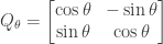


 , the rotation of all vectors in the x-y plane through the angle
  . We therefore have
  .
.
