Exercise 2.5.15. Suppose that MIT, Harvard, Yale, and Princeton compete in some sport, with MIT beating Harvard 35-0, Yale and Harvard playing to a tie, and Princeton beating Yale 7-6. What score differences in the other three possible games (MIT-Yale, MIT-Princeton, and Harvard-Princeton) would allow potential differences agreeing with the score differences?
Answer: We can consider this as a graph with four nodes (M, H, Y, and P) and six edges. Note that we can picture the nodes arranged in a square, with the edges M-H, H-Y, and Y-P forming three of the outside edges of the square, P-M forming the fourth outside edge, and Y-M and P-H being the diagonals. Note that we assume that each edge goes from the visiting team to the home team; thus, for example, the edge M-H represents a game played by MIT at Harvard.
The scores provided correspond to potential differences between the nodes, more specifically the potential of the home team minus the potential of the visiting team, which in our model corresponds to the score difference between the teams. Thus the potential difference 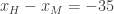 , the potential difference
  , and the potential difference
  .
.
The total potential differences around any loop must sum to 0; in particular this is true for the outer loop formed by the four edges of the square, so that


This potential difference is consistent with MIT beating Princeton by a score of 34-0, or 41-7, or any other score where MIT wins by 34 points.
Around the inner loop formed by the edges M-H, H-Y, and Y-M we have


This potential difference is consistent with MIT beating Yale by a score of 35-0, or 44-9, or any other score where MIT wins by 35 points.
Finally, around the inner loop formed by the edges P-H, H-Y, and Y-P we have


This potential difference is consistent with Princeton beating Harvard by a score of 7-6, or 14-13, or any other score where Princeton wins by 1 point.
Note also that the three edges M-H, H-Y, and Y-P form a spanning tree, since they connect all four nodes, and the score differences along those edges determine the score differences along all the other edges. This is true in general: If a set of edges forms a spanning tree, then the potential differences along those edges determine the potential differences along all other edges.
This occurs because a spanning tree is a graph that connects all the nodes but that has no loops. If another edge is added then that will form a loop where previously there was none, and since the potential differences around the new loop must sum to 0, the potential differences along the new edge are determined by the potential differences along the edges previously in the spanning tree.
NOTE: This continues a series of posts containing worked out exercises from the (out of print) book Linear Algebra and Its Applications, Third Edition by Gilbert Strang.
If you find these posts useful I encourage you to also check out the more current Linear Algebra and Its Applications, Fourth Edition , Dr Strang’s introductory textbook Introduction to Linear Algebra, Fourth Edition
 and the accompanying free online course, and Dr Strang’s other books
 .
.
 Buy me a snack to sponsor more posts like this!

axis
axis


 and transform it into the vector
 nodes, where every node has a edge connecting it to every other node. How many edges are in this complete graph?
 other nodes. This would normally produce a total of
  connections; however in order to avoid double counting a given edge we have to divide this value by 2. (In other words an edge from node
  to node
  counts as a connection for both nodes.) The total number of edges in the complete graph is therefore
  .
. edge, a 3-node complete graph has
  edges, a 4-node complete graph has
  edges, and so on.
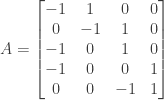
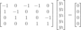
 expressed in matrix form as
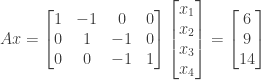

 then from the third equation we have
  . Substituting the value of
  into the second equation we have
  . Finally, substituting the value of
  into the first equation we have
  .
. at the three ungrounded nodes 1, 2, and 3.
 .
.

 . It can be derived from the three equations above by adding the first equation to the second equation to produce the equation
  and then adding this equation to the third equation to produce
  or
or 

 ,
,  , and
, and  are basic variables and
  and
and  are free variables. The resulting echelon matrix corresponds to the following system of equations:
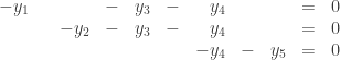
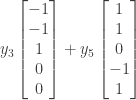
 and
and  then from the third equation we have
  . Substituting into the second equation we have
  . Substituting into the first equation we have
  .
. and
and  then from the third equation we have
  . Substituting into the second equation we have
  . Substituting into the first equation we have
  .
.
 from node 2 to node 3, equivalent to a current of
  from node 1 to node 4, equivalent to a current of
 and
and  have
have  rows
rows and
and  have
have  rows
rows and
and  have
have  rows
rows and
and  have
have  rows
rows
 is
is  is
is  is
is  is
is 

