Exercise 2.4.3. For each of the two matrices below give the dimension and find a basis for each of their four subspaces:
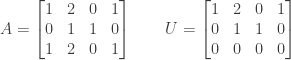
Answer: We first consider the column spaces  and
and  . The matrix
  has two pivots and therefore rank
  ; this is the dimension of the column space of . Since the pivots are in the first and second columns those columns are a basis for :

Note that the third column of is equal to -2 times the first column plus the second column, and the fourth column is equal to the first column.
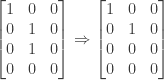
Doing Gaussian elimination on the matrix  (i.e., by subtracting the first row from the third) produces , so the rank of and the dimension of the column space of are also 2. Also, since the first and second columns of (the pivot columns) are a basis for the first and second columns of are a basis for :

Note that as with the third column of is equal to -2 times the first column plus the second column, and the fourth column is equal to the first column.
Turning to the row spaces, since the rows of are linear combinations of the rows of and vice versa, the row spaces  and
and  are the same. Per the discussion on page 91 the nonzero rows of , the vectors
  and
and  , form a basis for . Since
 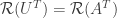 these vectors also form a basis for . The dimension of each row space is 2.
We now turn to the nullspaces  and
and  consisting of the solutions to the equations
  and
and  respectively. As noted above, if we do Gaussian elimination on (i.e., by subtracting the first row from the third row) then we obtain the matrix so that any solution to is a solution to and vice versa. We therefore have
 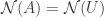 and just need to calculate one of the two.
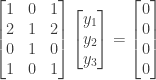
In particular for we must find  such that

Since the pivots of are in the first and second columns we have  and
and  as basic variables and
  and
and  as free variables.
From the second row of the system above we have  or
or  . From the first row we then have
  or
or  . Setting each of the free variables and to 1 in turn (and the other free variable to zero) we have the following set of vectors as solutions to the homogeneous equation and a basis for the null space of :

Since 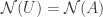 the above vectors also form a basis for the nullspace of . The dimension of the two nullspaces and is 2 (the number of columns of each matrix minus the rank, or
  ).
).
Finally we turn to finding a basis for each of the left nullspaces  and
and  . As discussed on page 95 there are two possible approaches to doing this. One way to find the left nullspace of is to look at the operations on the rows of needed to produce zero rows in the resulting echelon matrix in the process of Gaussian elimination; the coefficients used to carry out those operations make up the basis vectors of the left nullspace .
In particular, the one and only zero row in is produced by subtracting the first row of from the third row of , with no contribution from the second row; the coefficients for this operation are -1 (for the first row), 0 (for the second row), and 1 (for the third). The vector

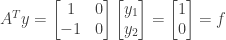
is therefore a basis for the left nullspace (which has dimension 1). We can test this by multiplying on the left by the transpose of this vector:

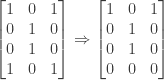
The left nullspace of can be found in a similar manner: Since is already in echelon form with a third row of zeroes, the step of Gaussian elimination to produce that row would be equivalent to multiplying the first row by zero and the second row by zero and then adding them to the third (zero) row; the coefficients for this operation are 0 (for the first row), 0 (for the second row), and 1 (for the third row). The vector

is therefore a basis for the left nullspace (which also has dimension 1). As with we can test this by multiplying on the left by the transpose of this vector:

An alternate approach to find the left nullspace of is to explicitly solve  or
or

Gaussian elimination on  proceeds as follows: First, subtract two times the first row from the second:

and then subtract the first row from the fourth row:

Finally, subtract the second row from the third row:
We thus have  and
and  as basic variables (since the pivots are in the first and second columns) and
  as a free variable. From the first row of the final matrix we have
  or
or  in the homogeneous case, and from the second row of the final matrix we have
  or
or  . Setting the free variable
  then gives us the vector
as a basis for the left nullspace of . The left nullspace of has dimension 1 (the number of rows of minus its rank, or  ).
).
Similarly we can also find the left nullspace of by solving the homogeneous system  or
or
Gaussian elimination on  proceeds as follows: First, subtract two times the first row from the second:

and then subtract the first row from the fourth row:
Finally, subtract the second row from the third row:

We thus have and as basic variables (since the pivots are in the first and second columns) and as a free variable. From the first row of the final matrix we have  or
or  in the homogeneous case, and from the second row of the final matrix we have or . Setting the free variable then gives us the vector
as a basis for the left nullspace of . As with the left nullspace of has dimension 1 (the number of rows of minus its rank, or ).
As with exercise 2.4.2, note that the row space of is equal to the row space of because the rows of are linear combinations of the rows of and vice versa. Similarly the nullspace of is equal to the nullspace of for the same reason.
UPDATE: Corrected two typos involving the equations for the left nullspace; thanks to Lucas for finding the errors.
NOTE: This continues a series of posts containing worked out exercises from the (out of print) book Linear Algebra and Its Applications, Third Edition by Gilbert Strang.
If you find these posts useful I encourage you to also check out the more current Linear Algebra and Its Applications, Fourth Edition , Dr Strang’s introductory textbook Introduction to Linear Algebra, Fourth Edition
 and the accompanying free online course, and Dr Strang’s other books
 .
.
 Buy me a snack to sponsor more posts like this!


 the system
  always has at least one solution. Show that in this case the system
  .
. .
. for any
  then the columns of
  . (The rank cannot be less than
  such that
  where
where  . The only element of
  in
in  for which
  . Find a 1 by 3 matrix
  with the same nullspace.
 and
and  . We know that
  ,
,  , and
, and  so that
  .
. each row of
  for
for  . Since
  or to any multiple of that vector. For example, one possible choice of
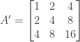
 is a linear combination of the columns of
  . If the only time when
  are all zero) then all the columns of
  .
. ? If not, why not?
 for
for  .
.
 .
. . For the left side we have


 existing such that
  ?
? such that
  we must have
  . Per the same theorem, for
  such that
  we must have
  . For
. For  , in which case
  .
. .
. and
and  are the columns of
 not to
 . But if that is the case then the vector
  is a solution to
  for two matrices
  is contained within the nullspace
  .
. matrix, and that
  are the columns of
  for all
  . In other words, each
  is in the nullspace of
  by any vector in the column space of
 and thus


 be the rows of
  for all
  is in the left nullspace of
  by any vector in the row space of


 . The row space is the y-z plane in
 and from the first row we have
  . Setting the free variable
 . In general we can find the left nullspace by looking at the operations on the rows of
 or
or

