My Math Homework

Linear Algebra and Its Applications, Exercise 2.4.2

Posted on April 23, 2012 by hecker

Exercise 2.4.2. For each of the two matrices below give the dimension and find a basis for each of their four subspaces:

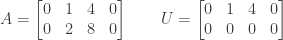
$A = \begin{bmatrix} 0&1&4&0 \\ 0&2&8&0 \end{bmatrix} \qquad U = \begin{bmatrix} 0&1&4&0 \\ 0&0&0&0 \end{bmatrix}$

Answer: The echelon matrix $U$ has only a single pivot, in the second column. As discussed on page 93, the second column $\begin{bmatrix} 1 \\ 0 \end{bmatrix}$ is therefore a basis for the column space $\mathcal{R}(U)$ . (The third column of $U$ is equal to four times the second column.) The dimension of $\mathcal{R}(U)$ is 1 (same as the rank of $U$ ).

The echelon matrix $U$ can be derived from $A$ via Gaussian elimination (i.e., by subtracting two times the first row of $A$ from the second row of $A$ ). Again per the discussion on page 93, since the second column of $U$ is a basis for the column space of $U$ the second column of $A$ , the vector $\begin{bmatrix} 1 \\ 2 \end{bmatrix}$ , is a basis for the column space of $A$ . (As with $U$ , the third column of $A$ is equal to four times the second column.) The dimension of $\mathcal{R}(A)$ is 1 (the same as the rank of $A$ , which is the same as the rank of $U$ ).

Turning to the row spaces, the only nonzero row of the echelon matrix $U$ is the first row, so per the discussion on page 91 the vector $\begin{bmatrix} 0,&1&4&0 \end{bmatrix}^T$ is a basis for the row space $\mathcal{R}(U^T)$ . The dimension of $\mathcal{R}(U^T)$ is 1 (again, the same as the rank of $U$ ). Since the matrix $U$ can be derived from $A$ using Gaussian elimination the row spaces of the two matrices are identical, so that the vector $\begin{bmatrix} 0,&1&4&0 \end{bmatrix}^T$ is also a basis for the row space $\mathcal{R}(A^T)$ . (This basis vector happens to be the first row of $A$ , and the second row of $A$ is equal to two times the first row.) The dimension of $\mathcal{R}(A^T)$ is 1 (same as the rank of $A$ and $U$ ).

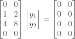
We now turn to the nullspaces $\mathcal N(A)$ and $\mathcal N(U)$ , i.e., the solutions to the equations $Ax = 0$ and $Ux = 0$ . In particular for $Ux = 0$ we must find $x = (x_1, x_2, x_3, x_4)$ such that

$\begin{bmatrix} 0&1&4&0 \\ 0&0&0&0 \end{bmatrix} \begin{bmatrix} x_1 \\ x_2 \\ x_3 \\ x_4 \end{bmatrix} = 0$

As noted above, if we do Gaussian elimination on $A$ (i.e., by multiplying the first row by 2 and subtracting it from the second row) then we obtain the matrix $U$ . Both matrices thus have rank $r = 1$ with $x_2$ being a basic variable (since the pivot is in the second column) and $x_1$ , $x_3$ , and $x_4$ being free variables.

From the equation above we see that we must have $x_2 + 4x_3 = 0$ or $x_2 = -4x_3$ . Setting each of the free variables $x_1$ , $x_3$ , and $x_4$ to 1 in turn (with the other free variables set to zero) we have the following set of vectors as solutions to the homogeneous equation $Ux = 0$ and a basis for the null space of $U$ :

$\begin{bmatrix} 1 \\ 0 \\ 0 \\ 0 \end{bmatrix} \qquad \begin{bmatrix} 0 \\ -4 \\ 1 \\ 0 \end{bmatrix} \qquad \begin{bmatrix} 0 \\ 0 \\ 0 \\ 1 \end{bmatrix}$

Since $U$ can be obtained from $A$ by Gaussian elimination any solution to $Ax = 0$ is also a solution to $Ux = 0$ and vice versa, so the above vectors also form a basis for the nullspace of $A$ . The dimensions of the two nullspaces $\mathcal N(U)$ and $\mathcal N(A)$ are both 3 (equal to the number of vectors in the basis) and in fact the nullspaces are identical (since they have the exact same basis).

Finally we turn to finding a basis for each of the left nullspaces $\mathcal N(A^T)$ and $\mathcal N(U^T)$ . As discussed on page 95 there are two possible approaches to doing this. One way to find the left nullspace of $A$ is to look at the operations on the rows of $A$ needed to produce zero rows in the resulting echelon matrix $U$ in the process of Gaussian elimination; the coefficients used to carry out those operations make up the basis vectors of the left nullspace $\mathcal N(A^T)$ .

In particular, the one and only zero row in $U$ is produced by multiplying the first row of $A$ by two and subtracting it from the second row of $A$ ; the coefficients for this operation are -2 (for the first row) and 1 (for the second). The vector $\begin{bmatrix} -2 \\ 1 \end{bmatrix}$ is therefore a basis for the left nullspace $\mathcal N(A^T)$ (which has dimension 1). We can test this by multiplying $A$ on the left by the transpose of this vector:

$\begin{bmatrix} -2&1 \end{bmatrix} \begin{bmatrix} 0&1&4&0 \\ 0&2&8&0 \end{bmatrix} = \begin{bmatrix} 0&0&0&0 \end{bmatrix}$

The left nullspace of $U$ can be found in a similar manner: Since $U$ is already in echelon form the first step of Gaussian elimination would be equivalent to adding nothing to the second row, in other words, multiplying the first row by zero and then adding it to the second (zero) row; the coefficients for this operation are 0 (for the first row) and 1 (for the second). The vector $\begin{bmatrix} 0 \\ 1 \end{bmatrix}$ is therefore a basis for the left nullspace $\mathcal N(U^T)$ (which also has dimension 1). As with $A$ we can test this by multiplying $U$ on the left by the transpose of this vector:

$\begin{bmatrix} 0&1 \end{bmatrix} \begin{bmatrix} 0&1&4&0 \\ 0&0&0&0 \end{bmatrix} = \begin{bmatrix} 0&0&0&0 \end{bmatrix}$

An alternate approach to find the left nullspace of $U$ is to explicitly solve $U^Ty = 0$ or

$\begin{bmatrix} 0&0 \\ 1&0 \\ 4&0 \\ 0&0 \end{bmatrix} \begin{bmatrix} y_1 \\ y_2 \end{bmatrix} = \begin{bmatrix} 0&0 \\ 0&0 \\ 0&0 \\ 0&0 \end{bmatrix}$

Gaussian elimination on $U^T$ proceeds as follows, first by exchanging the first row and second row and then by subtracting 4 times the first row from the third:

$\begin{bmatrix} 0&0 \\ 1&0 \\ 4&0 \\ 0&0 \end{bmatrix} \Rightarrow \begin{bmatrix} 1&0 \\ 0&0 \\ 4&0 \\ 0&0 \end{bmatrix} \Rightarrow \begin{bmatrix} 1&0 \\ 0&0 \\ 0&0 \\ 0&0 \end{bmatrix}$

We thus have $y_1$ as a basic variable (since the pivot is in the first column) and $y_2$ as a free variable. From the first row of the final matrix we have $1 \cdot y_1 + 0 \cdot y_2 = 0$ or $y_1 = 0$ in the homogeneous case. Setting the free variable $y_2 = 1$ then gives us the vector $\begin{bmatrix} 0 \\ 1 \end{bmatrix}$ as a basis for the left nullspace of $U$ . Since there is only one vector in the basis the left nullspace of $U$ has dimension 1.

Similarly we can also find the left nullspace of $A$ by solving the homogeneous system $A^Ty = 0$ or

$\begin{bmatrix} 0&0 \\ 1&2 \\ 4&8 \\ 0&0 \end{bmatrix} \begin{bmatrix} y_1 \\ y_2 \end{bmatrix} = \begin{bmatrix} 0&0 \\ 0&0 \\ 0&0 \\ 0&0 \end{bmatrix}$

Gaussian elimination on $A^T$ proceeds as follows, first by exchanging the first row and second row and then by subtracting 4 times the first row from the third:

$\begin{bmatrix} 0&0 \\ 1&2 \\ 4&8 \\ 0&0 \end{bmatrix} \Rightarrow \begin{bmatrix} 1&2 \\ 0&0 \\ 4&8 \\ 0&0 \end{bmatrix} \Rightarrow \begin{bmatrix} 1&2 \\ 0&0 \\ 0&0 \\ 0&0 \end{bmatrix}$

As with $U^Ty = 0$ we have $y_1$ as a basic variable and $y_2$ as a free variable. From the first row of the final matrix we have $1 \cdot y_1 + 2 \cdot y_2 = 0$ or $y_1 = -2y_1$ in the homogeneous case. Setting the free variable $y_2 = 1$ then gives us the vector $\begin{bmatrix} -2 \\ 1 \end{bmatrix}$ as a basis for the left nullspace of $A$ . Since there is only one vector in the basis the left nullspace of $A$ has dimension 1.

Note that the dimension of the column space of $A$ is the rank $r$ of $A$ , namely 1, while the dimension of the nullspace of $A$ is equal to the number of columns of $A$ minus the rank, or $n - r = 4 - 1 = 3$ . The dimension of the row space of $A$ is also $r = 1$ while the dimension of the left nullspace of $A$ is equal to the number of rows of $A$ minus the rank, or $m - r = 2 - 1 = 1$ . These results are in accordance with the Fundamental Theorem of Linear Algebra, Part I on page 95. Similar results hold for $U$ .

Also note that the row space of $A$ is equal to the row space of $U$ ; this is because the rows of $A$ are linear combinations of the rows of $U$ and vice versa. Similarly the nullspace of $A$ is equal to the nullspace of $U$ for the same reason.

NOTE: This continues a series of posts containing worked out exercises from the (out of print) book Linear Algebra and Its Applications, Third Edition by Gilbert Strang.

If you find these posts useful I encourage you to also check out the more current Linear Algebra and Its Applications, Fourth Edition, Dr Strang’s introductory textbook Introduction to Linear Algebra, Fourth Edition and the accompanying free online course, and Dr Strang’s other books.

Buy me a snack to sponsor more posts like this!

Posted in linear algebra | Tagged basis, dimension, fundamental subspaces | Leave a comment

Linear Algebra and Its Applications, Exercise 2.4.1

Posted on April 16, 2012 by hecker

Exercise 2.4.1. Suppose that for an $m$ by $n$ matrix $A$ we have $m = n$ . State whether the following is true or false: The row space $\mathcal{R}(A^T)$ and column space $\mathcal{R}(A)$ of $A$ are the same.

Answer: Consider the following example of a 2 by 2 echelon matrix $U$ with a single pivot:

$U = \begin{bmatrix} 1&2 \\ 0&0 \end{bmatrix}$

Since the second row is zero the first row is the only vector contributing to the row space $\mathcal{R}(U^T)$ and thus the vector $\begin{bmatrix} 1 \\ 2 \end{bmatrix}$ is a basis for $\mathcal{R}(U^T)$ . In geometric terms the row space $\mathcal{R}(U^T)$ is the line represented by the equation $y = 2x$ .

Since the only pivot is in the first column that column $\begin{bmatrix} 1 \\ 0 \end{bmatrix}$ is a basis for the column space $\mathcal{R}(U)$ . In geometric terms the column space $\mathcal{R}(U)$ is the x-axis.

So the row space $\mathcal{R}(U^T)$ and column space $\mathcal{R}(U)$ are not equal for this example matrix $U$ , even though the number of rows $m$ of $U$ is the same as the number of columns $n$ . The statement above is therefore false.

NOTE: This continues a series of posts containing worked out exercises from the (out of print) book Linear Algebra and Its Applications, Third Edition by Gilbert Strang.

Buy me a snack to sponsor more posts like this!

Posted in linear algebra | Leave a comment

Linear Algebra and Its Applications, Exercise 2.3.23

Posted on September 27, 2011 by hecker

Exercise 2.3.23. Let $v_1$ through $v_9$ be vectors in $\mathbf{R}^7$ . Answer the following questions:

a) Are the nine vectors linearly independent? Not linearly independent? Might be linearly independent?

b) Do the nine vectors span $\mathbf{R}^7$ ? Not span $\mathbf{R}^7$ ? Might span $\mathbf{R}^7$ ?

c) Suppose the nine vectors are the columns of a matrix $A$ . Does $Ax = b$ have a solution? Not have a solution? Might have a solution?

Answer: a) We cannot have a set of 9 linearly independent vectors in a space like $\mathbf{R}^7$ that has dimension 7. So the vectors are not linearly independent.

b) The vectors might or might not span $\mathbf{R}^7$ . For example, consider the set of vectors $(1, 0, 0, 0, 0, 0, 0)$ , $(2, 0, 0, 0, 0, 0, 0)$ , through $(9, 0, 0, 0, 0, 0, 0)$ . The nine vectors do not span $\mathbf{R}^7$ but rather span a subspace of dimension 1.

c) The matrix $A$ would have nine columns but only seven rows, and would correspond to a system of seven linear equations with nine unknowns. This system could not have more than seven basic variables and thus would have at least two free variables. Since the free variables can take on any value the system $Ax = 0$ is guaranteed to have a solution (and in fact would have an infinite number of them) but the system $Ax = b$ might or might not have a solution depending on the value of $b$ .

NOTE: This continues a series of posts containing worked out exercises from the (out of print) book Linear Algebra and Its Applications, Third Edition by Gilbert Strang.

Posted in linear algebra | 1 Comment

Linear Algebra and Its Applications, Exercise 2.3.22

Posted on September 26, 2011 by hecker

Exercise 2.3.22. Given a vector space $V$ of dimension 7 and a subspace $W$ of $V$ of dimension 4, state whether the following are true or false:

1) You can create a basis for $V$ by adding three vectors to any set of vectors that is a basis for $W$ .

2) You can create a basis for $W$ by removing three vectors from any set of vectors that is a basis for $V$ .

Answer: 1) True. Suppose $w_1$ , $w_2$ , $w_3$ , and $w_4$ are a basis for $W$ . Per 2L (page 86) any linearly independent set in $V$ can be extended to a basis for $V$ by adding more vectors if necessary. The four vectors $w_1$ through $w_4$ are already linearly independent (since they are a basis) and hence can be extended by adding additional vectors to form a basis for $V$ .

More specifically, we can find three vectors $v_1$ , $v_2$ , and $v_3$ such that a) the three vectors are not in $W$ (and hence are linearly independent of $w_1$ through $w_4$ ), and b) the three vectors are linearly independent of each other. The resulting seven vectors are linearly independent. Since the dimension of $V$ is 7 these seven linearly independent vectors must be a basis for $V$ . (See exercise 2.3.15.)

2) False. Consider the vectors $v_1 = (1, 0, 0, 0, 0, 0, 0)$ through $v_7 = (0, 0, 0, 0, 0, 0, 1)$ with $v_i$ having a one in the $i^{th}$ position and zeros elsewhere. These vectors are linearly independent and span $V$ and hence are a basis for it.

Now suppose $W$ is the subspace of all vectors of the form $(a, a, b, b, c, c, d)$ . The vectors $v_1$ through $v_6$ are not in the subspace $W$ and hence cannot be part of a basis for it. Thus it is not possible to remove three vectors from the basis set $v_1$ through $v_7$ and form a basis for $W$ .

NOTE: This continues a series of posts containing worked out exercises from the (out of print) book Linear Algebra and Its Applications, Third Edition by Gilbert Strang.

Posted in linear algebra | Leave a comment

Linear Algebra and Its Applications, Exercise 2.3.21

Posted on September 25, 2011 by hecker

Exercise 2.3.21. Suppose $A$ is a 64 by 17 matrix and has rank 11. How many independent vectors are solutions to the system $Ax = 0$ ? What about the system $A^Ty = 0$ ?

Answer: If the rank of $A$ is 11 then performing elimination on $A$ produces an matrix $U$ with 11 pivots and thus 11 basic variables. Since $U$ (like $A$ ) has 17 columns this means that there are 17 – 11 or 6 free variables that can be set to arbitrary values in solving the system $Ax = 0$ . The nullspace of $A$ (i.e., the set of all vectors satisfying $Ax = 0$ ) therefore has dimension 6, and any basis for the nullspace has 6 linearly independent vectors each of which satisfy $Ax = 0$ .

Since $A$ is 64 by 17 the matrix $A^T$ is 17 by 64. The original matrix $A$ had 11 pivots and 11 linearly independent rows. The rows of $A$ become columns in $A^T$ and thus $A^T$ has 11 linearly independent columns and also has rank 11. Since $A^T$ has 64 columns there are 64 – 11 or 53 free variables when considering the system $A^Ty = 0$ . The nullspace of $A^T$ (i.e., the set of all vectors satisfying $A^Ty = 0$ ) therefore has dimension 53, and any basis for the nullspace has 53 linearly independent vectors each of which satisfy $A^Ty = 0$ .

NOTE: This continues a series of posts containing worked out exercises from the (out of print) book Linear Algebra and Its Applications, Third Edition by Gilbert Strang.

Posted in linear algebra | Leave a comment

Linear Algebra and Its Applications, Exercise 2.3.20

Posted on September 24, 2011 by hecker

Exercise 2.3.20.Consider the set of all 2 by 2 matrices that have the sum of their rows equal to the sum of their columns. What is a basis for this subspace? Consider the analogous set of 3 by 3 matrices with equal row and column sums. List five linearly independent matrices from this set.

Answer: Any 2 by 2 matrix $A$ in the set will have the form

$A = \begin{bmatrix} a&b \\ b&a \end{bmatrix}$

with the sum of every row and every column being $a+b$ . Any such matrix $A$ can be represented as a linear combination of two matrices as follows:

$A = a \begin{bmatrix} 1&0 \\ 0&1 \end{bmatrix} + b \begin{bmatrix} 0&1 \\ 1&0 \end{bmatrix}$

Since the two matrices are linearly independent and span the subspace they are a basis for the subspace.

The following five matrices are linearly independent members of the analogous set for 3 by 3 matrices:

$\begin{bmatrix} 1&0&0 \\ 0&1&0 \\ 0&0&1 \end{bmatrix} \quad \begin{bmatrix} 0&1&0 \\ 0&0&1 \\ 1&0&0 \end{bmatrix} \quad \begin{bmatrix} 0&0&1 \\ 1&0&0 \\ 0&1&0 \end{bmatrix}$

$\begin{bmatrix} 0&1&0 \\ 1&0&0 \\ 0&0&1 \end{bmatrix} \quad \begin{bmatrix} 1&0&0 \\ 0&0&1 \\ 0&1&0 \end{bmatrix}$

NOTE: This continues a series of posts containing worked out exercises from the (out of print) book Linear Algebra and Its Applications, Third Edition by Gilbert Strang.

Posted in linear algebra | Leave a comment

Linear Algebra and Its Applications, Exercise 2.3.19

Posted on September 23, 2011 by hecker

Exercise 2.3.19. Suppose $A$ is an $m$ by $n$ matrix, with $n$ columns taken from $\mathbf{R}^m$ . What is the rank of $A$ if its column vectors are linearly independent? What is the rank of $A$ if its column vectors span $\mathbf{R}^m$ ? What is the rank of $A$ if its column vectors are a basis for $\mathbf{R}^m$ ?

Answer: If the $n$ column vectors of $A$ are linearly independent then there must be a pivot in every one of the $n$ columns, so that the rank $r = n$ .

If the $n$ columns of $A$ span $\mathbf{R}^m$ then we must have $n \ge m$ . There can be no more than $m$ linearly independent vectors in $\mathbf{R}^m$ so out of the $n$ columns of $A$ only $m$ columns can have pivots. Therefore the rank $r = m$ .

If the $n$ columns of $A$ are a basis for $\mathbf{R}^m$ then they are linearly independent, which means the rank $r = n$ , and they also span $\mathbf{R}^m$ so we must also have $r = m$ . We thus have $r = m = n$ .

NOTE: This continues a series of posts containing worked out exercises from the (out of print) book Linear Algebra and Its Applications, Third Edition by Gilbert Strang.

Posted in linear algebra | Leave a comment

Linear Algebra and Its Applications, Exercise 2.3.18

Posted on September 22, 2011 by hecker

Exercise 2.3.18. Indicate whether the following statements are true or false:

a) given a matrix $A$ whose columns are linearly independent, the system $Ax = b$ has one and only solution for any right-hand side $b$

b) if $A$ is a 5 by 7 matrix then the columns of $A$ cannot be linearly independent

Answer: a) False. If $A$ has fewer columns than rows then the system $Ax = b$ has more equations than unknowns and may not have a solution. For example, if

$A = \begin{bmatrix} 1&0 \\ 0&1 \\ 0&1 \end{bmatrix} \quad \rm and \quad b = \begin{bmatrix} 0 \\ 0 \\ 1 \end{bmatrix}$

corresponding to the system

$\setlength\arraycolsep{0.2em}\begin{array}{rcrcl}x_1&&&=&0 \\ &&x_2&=&0 \\ &&x_2&=&1 \end{array}$

then the columns of $A$ are linearly independent but the system $Ax = b$ has no solution since the second and the third equations result in a contradiction.

b) True. If $A$ is a 5 by 7 matrix then it has seven columns, each of which is an element of $\mathbf{R}^5$ . But it is impossible to have more than five linearly independent vectors in $\mathbf{R}^5$ so the columns of $A$ must be linearly dependent.

NOTE: This continues a series of posts containing worked out exercises from the (out of print) book Linear Algebra and Its Applications, Third Edition by Gilbert Strang.

Posted in linear algebra | Leave a comment

Linear Algebra and Its Applications, Exercise 2.3.17

Posted on September 21, 2011 by hecker

Exercise 2.3.17. Suppose that $V$ and $W$ are subspaces of $\mathbf{R}^5$ , each with dimension 3. Show that $V$ and $W$ must have at least one vector in common other than the zero vector.

Answer: Since $V$ and $W$ each have dimension 3 their respective bases each contain three vectors. Let $v_1$ , $v_2$ , and $v_3$ be a basis for $V$ and $w_1$ , $w_2$ , and $w_3$ be a basis for $W$ .

Now consider the combined set of six vectors. Since we have six vectors in a vector space of dimension 5 the combined set of vectors is linearly dependent, with at least one vector expressible as a linear combination of the other five vectors. Without loss of generality assume that $w_3$ is dependent on the other five vectors, so that we have

$w_3 = c_1v_1 + c_2v_2 + c_3v_3 + c_4w_1 + c_5w_2$

for some set of weights $c_1$ through $c_5$ . We can rearrange the above equation as follows:

$c_1v_1 + c_2v_2 + c_3v_3 = -c_4w_1 - c_5w_2 + w_3$

Now consider the vector $u = c_1v_1 + c_2v_2 + c_3v_3$ . Since $u$ is a linear combination of the basis vectors $v_1$ , $v_2$ , and $v_3$ it is in the subspace $V$ . But from the above equation we also have $u = -c_4w_1 - c_5w_2 + w_3$ so that $u$ is a linear combination of the basis vectors $w_1$ , $w_2$ , and $w_3$ and thus is also in the subspace $W$ .

So $u$ is a member of both $V$ and $W$ . Now suppose $u = 0$ . We then have $-c_4w_1 - c_5w_2 + w_3 = 0$ or $w_3 = c_4w_1 + c_5w_2$ so that $w_3$ is a linear combination of $w_1$ and $w_2$ and the set of vectors $w_1$ , $w_2$ , and $w_3$ is linearly dependent. But this contradicts the assumption that $w_1$ , $w_2$ , and $w_3$ form a basis for $W$ and are thus linearly independent. Since the assumption $u = 0$ leads to a contradiction we conclude that $u \ne 0$ .

We have thus shown that there must exist a nonzero vector $u$ that is a member of both $V$ and $W$ .

NOTE: This continues a series of posts containing worked out exercises from the (out of print) book Linear Algebra and Its Applications, Third Edition by Gilbert Strang.

Posted in linear algebra | Leave a comment

Linear Algebra and Its Applications, Exercise 2.3.16

Posted on September 20, 2011 by hecker

Exercise 2.3.16. What is the dimension of the vector space consisting of all 3 by 3 symmetric matrices? What is a basis for it?

Answer: There are nine possible entries that can be set in a 3 b 3 matrix, but if the matrix is symmetric then only six of them can be set independently, since we must have $a_{12} = a_{21}$ , $a_{13} = a_{31}$ , and $a_{23} = a_{32}$ . Any symmetric matrix

$A = \begin{bmatrix} a_{11}&a_{12}&a_{13} \\ a_{12}&a_{22}&a_{23} \\ a_{13}&a_{23}&a_{33} \end{bmatrix}$

can be represented as a linear combination of six linearly independent matrices as follows:

$A = a_{11} \begin{bmatrix} 1&0&0 \\ 0&0&0 \\ 0&0&0 \end{bmatrix} + a_{22} \begin{bmatrix} 0&0&0 \\ 0&1&0 \\ 0&0&0 \end{bmatrix} + a_{33} \begin{bmatrix} 0&0&0 \\ 0&0&0 \\ 0&0&1 \end{bmatrix}$

$+ a_{12} \begin{bmatrix} 0&1&0 \\ 1&0&0 \\ 0&0&0 \end{bmatrix} + a_{13} \begin{bmatrix} 0&0&1 \\ 0&0&0 \\ 1&0&0 \end{bmatrix} + a_{23} \begin{bmatrix} 0&0&0 \\ 0&0&1 \\ 0&1&0 \end{bmatrix}$

Since the above set of six linearly independent matrices spans the space of 3 by 3 symmetric matrices it is a basis for the space, and the dimension of the space is therefore six.

UPDATE: Corrected a typo in the definition of the matrix $A$ . Thanks go to James Teow for finding this error.

NOTE: This continues a series of posts containing worked out exercises from the (out of print) book Linear Algebra and Its Applications, Third Edition by Gilbert Strang.

Posted in linear algebra | 2 Comments

My Math Homework

Linear Algebra and Its Applications, Exercise 2.4.2

Linear Algebra and Its Applications, Exercise 2.4.1

Linear Algebra and Its Applications, Exercise 2.3.23

Linear Algebra and Its Applications, Exercise 2.3.22

Linear Algebra and Its Applications, Exercise 2.3.21

Linear Algebra and Its Applications, Exercise 2.3.20

Linear Algebra and Its Applications, Exercise 2.3.19

Linear Algebra and Its Applications, Exercise 2.3.18

Linear Algebra and Its Applications, Exercise 2.3.17

Linear Algebra and Its Applications, Exercise 2.3.16

Archives

Meta