Linear Algebra and Its Applications, exercise 1.4.3

Exercise 1.4.3. Multiply the matrices below:

\begin{bmatrix} 1&-2&7 \end{bmatrix}  \begin{bmatrix} 1 \\ -2 \\ 7 \end{bmatrix} \rm and \begin{bmatrix} 1&-2&7 \end{bmatrix}  \begin{bmatrix} 3 \\ 5  \\ 1 \end{bmatrix} \rm and \begin{bmatrix} 1 \\ -2 \\ 7 \end{bmatrix} \begin{bmatrix} 3&5&1 \end{bmatrix}

Answer: The first example multiplies a 1×3 matrix by a 3×1 matrix producing a 1×1 matrix, i.e., a scalar value:

1 \cdot 1 + (-2) \cdot (-2) + 7 \cdot 7 = 1 + 4 + 49 = 54

As noted in the book, the result is equal to the square of the length of the vector (1, -2, 7) .

For the second example we’re also multiplying a 1×3 matrix times a 3×1 matrix to produce a scalar value:

1 \cdot 3 + (-2) \cdot 5 + 7 \cdot 1 = 3 - 10 + 7 = 0

The final example multiplies a 3×1 matrix times a 1×3 matrix to produce a 3×3 matrix:

\begin{bmatrix} 1 \\ -2 \\ 7 \end{bmatrix}  \begin{bmatrix} 3&5&1 \end{bmatrix} = \begin{bmatrix} 1 \cdot 3&1 \cdot 5&1 \cdot 1 \\ -2 \cdot 3&-2 \cdot 5&-2 \cdot 1 \\ 7 \cdot 3&7 \cdot 5&7 \cdot 1  \end{bmatrix} = \begin{bmatrix} 3&5&1 \\ -6&-10&-2 \\ 21&35&7 \end{bmatrix}

NOTE: This continues a series of posts containing worked out exercises from the (out of print) book Linear Algebra and Its Applications, Third Edition by Gilbert Strang.

If you find these posts useful I encourage you to also check out the more current Linear Algebra and Its Applications, Fourth Edition, Dr Strang’s introductory textbook Introduction to Linear Algebra, Fourth Edition and the accompanying free online course, and Dr Strang’s other books.

Posted in linear algebra | Leave a comment

Linear Algebra and Its Applications, exercise 1.4.2

Exercise 1.4.2. Multiply the matrices below:

\left[ \begin{array}{rr} 4&1 \\ 5&1 \\ 6&1 \end{array} \right] \left[ \begin{array}{r} 1 \\ 3  \end{array} \right] \rm and \left[ \begin{array}{rrr} 1&2&3 \\ 4&5&6 \\ 7&8&9 \end{array} \right] \left[  \begin{array}{r} 0 \\ 1 \\ 0 \end{array} \right] \rm and \left[  \begin{array}{rr} 4&3 \\ 6&6 \\ 8&9\end{array} \right] \left[  \begin{array}{r} \frac{1}{2} \\ \frac{1}{3}  \end{array} \right]

Work by columns instead of by rows.

Answer: The first example multiplies a 3×2 matrix by a 2×1 matrix (column vector), producing a 3×1 matrix (column vector). Working by rows gives us the following:

\left[ \begin{array}{rr} 4&1 \\ 5&1 \\ 6&1  \end{array} \right] \left[ \begin{array}{r} 1 \\ 3  \end{array} \right] = \left[ \begin{array}{r} 4 \cdot 1 + 1 \cdot 3 \\ 5 \cdot 1 + 1 \cdot 3 \\ 6 \cdot 1 + 1 \cdot 3  \end{array}  \right] = \left[ \begin{array}{r} 7 \\ 8 \\ 9  \end{array}  \right]

Working by columns is done as follows:

\begin{bmatrix} 4&1 \\ 5&1 \\ 6&1   \end{bmatrix} \begin{bmatrix} 1 \\ 3  \end{bmatrix} = \begin{bmatrix} 4 \\ 5 \\ 6  \end{bmatrix} \cdot 1 + \begin{bmatrix} 1 \\ 1  \\ 1  \end{bmatrix} \cdot 3 = \begin{bmatrix} 4 \\ 5  \\ 6  \end{bmatrix} + \begin{bmatrix} 3 \\ 3  \\ 3  \end{bmatrix} = \begin{bmatrix}  7 \\ 8 \\ 9  \end{bmatrix}

For the second example we’re multiplying a 3×3 matrix times a 3×1 matrix to produce a 3×1 matrix (column vector). Working by rows gives us the following:

\begin{bmatrix} 1&2&3 \\ 4&5&6 \\ 7&8&9 \end{bmatrix} \begin{bmatrix} 0 \\ 1 \\ 0 \end{bmatrix} = \begin{bmatrix} 1 \cdot 0 + 2 \cdot 1 + 3 \cdot 0 \\ 4 \cdot 0 + 5 \cdot 1 + 6 \cdot 0 \\ 7 \cdot 0 + 8 \cdot 1 + 9 \cdot 0 \end{bmatrix} = \begin{bmatrix} 2 \\ 5 \\ 8 \end{bmatrix}

Working by columns is done as follows:

\begin{bmatrix} 1&2&3 \\ 4&5&6 \\ 7&8&9  \end{bmatrix} \begin{bmatrix} 0 \\ 1 \\ 0 \end{bmatrix} = \begin{bmatrix} 1 \\ 4 \\ 7 \end{bmatrix} \cdot 0 + \begin{bmatrix} 2 \\ 5 \\ 8 \end{bmatrix} \cdot 1 + \begin{bmatrix} 3 \\ 6 \\ 9 \end{bmatrix} \cdot 0 = \begin{bmatrix} 0 \\ 0 \\ 0 \end{bmatrix} + \begin{bmatrix} 2 \\ 5 \\ 8 \end{bmatrix} + \begin{bmatrix} 0 \\ 0 \\ 0 \end{bmatrix} = \begin{bmatrix} 2 \\ 5 \\ 8 \end{bmatrix}

Note that this is a special case of the general case that multiplying an nxn matrix by a column vector of the form (0, …, 0, 1, 0, …, 0) (where the jth entry is 1 and the others zero) produces a column vector corresponding to the jth column of the matrix.

The third example multiplies a 3×2 matrix by a 2×1 matrix to form a 3×1 matrix. Working by rows gives us the following:

\begin{bmatrix} 4&3 \\ 6&6 \\ 8&9 \end{bmatrix} \begin{bmatrix} \frac{1}{2} \\ \frac{1}{3} \end{bmatrix} = \begin{bmatrix} 4 \cdot \frac{1}{2} + 3 \cdot \frac{1}{3} \\ 6 \cdot \frac{1}{2} + 6 \cdot \frac{1}{3} \\ 8 \cdot \frac{1}{2} + 9 \cdot \frac{1}{3} \end{bmatrix} = \begin{bmatrix} 2 + 1 \\ 3 + 2 \\ 4 + 3 \end{bmatrix} = \begin{bmatrix} 3 \\ 5 \\ 7 \end{bmatrix}

Working by columns is done as follows:

\begin{bmatrix} 4 \\ 6 \\ 8 \end{bmatrix} \cdot \frac{1}{2} + \begin{bmatrix} 3 \\ 6 \\ 9 \end{bmatrix} \cdot \frac{1}{3} = \begin{bmatrix} 2 \\ 3 \\ 4 \end{bmatrix} +  \begin{bmatrix} 1 \\ 2 \\ 3 \end{bmatrix} = \begin{bmatrix} 3 \\ 5 \\ 7 \end{bmatrix}

NOTE: This continues a series of posts containing worked out exercises from the (out of print) book Linear Algebra and Its Applications, Third Edition by Gilbert Strang.

If you find these posts useful I encourage you to also check out the more current Linear Algebra and Its Applications, Fourth Edition, Dr Strang’s introductory textbook Introduction to Linear Algebra, Fourth Edition and the accompanying free online course, and Dr Strang’s other books.

Posted in linear algebra | Leave a comment

Linear Algebra and Its Applications, exercise 1.4.1

Exercise 1.4.1. Multiply the matrices below:

\left[ \begin{array}{rrr} 4&0&1 \\ 0&1&0 \\ 4&0&1 \end{array} \right] \left[ \begin{array}{r} 3 \\ 4 \\ 5 \end{array} \right] \rm and \left[ \begin{array}{rrr} 1&0&0 \\ 0&1&0 \\ 0&0&1 \end{array} \right] \left[ \begin{array}{r} 5 \\ -2 \\ 3 \end{array} \right] \rm and \left[ \begin{array}{rr} 2&0 \\ 1&3 \end{array} \right] \left[ \begin{array}{r} 1 \\ 1  \end{array} \right]

(The exercise also asks you to draw a graph showing addition of the two vectors (2, 1) and (0, 3); I’m skipping that part.)

Answer: The first example multiplies a 3×3 matrix by a 3×1 matrix (column vector), producing a 3×1 matrix. The first entry in the resulting column vector is

4 \cdot 3 + 0 \cdot 4 + 1 \cdot 5 = 12 + 0 + 5 = 17

The second entry in the resulting column vector is

0  \cdot 3 + 1 \cdot 4 + 0 \cdot 5 = 0 + 4 + 0 = 4

The third entry in the resulting column vector is the same as the first entry:

4 \cdot 3 + 0 \cdot 4 + 1 \cdot 5 = 12 + 0 + 5 = 17

The column vector that is the product of the multiplication is therefore (17, 4, 17):

\left[ \begin{array}{rrr} 4&0&1 \\ 0&1&0 \\  4&0&1 \end{array} \right] \left[ \begin{array}{r} 3 \\ 4 \\ 5  \end{array} \right] = \left[ \begin{array}{r} 17 \\ 4 \\ 17  \end{array} \right]

For the second example we’re again multiplying a 3×3 matrix times a 3×1 matrix to produce 3×1 matrix (column vector). The three entries in the column vector are computed as follows:

1 \cdot 5 + 0 \cdot (-2) + 0 \cdot 3 = 5 + 0 + 0 = 5

0 \cdot 5 + 1 \cdot (-2) + 0 \cdot 3 = 0 - 2 + 0 = -2

0 \cdot 5 + 0 \cdot (-2) + 1 \cdot 3 = 0 + 0 + 3 = 3

The product is thus the column vector (5, -2, 3), and this is a special case of the general case IA = A where I is the identity matrix.

The third example multiplies a 2×2 matrix by a 2×1 matrix to form a 2×1 matrix, with entries as follows:

2 \cdot 1 + 0 \cdot 1 = 2 + 0 = 2

1 \cdot 1 + 3 \cdot 1 = 1 + 3 = 4

We therefore have

\left[ \begin{array}{rr} 2&0 \\ 1&3 \end{array} \right] \left[  \begin{array}{r} 1 \\ 1  \end{array} \right] = \left[  \begin{array}{r} 2 \\ 4  \end{array} \right]

Note that we also have

\left[  \begin{array}{r} 2 \\ 1  \end{array} \right] + \left[  \begin{array}{r} 0 \\ 3  \end{array} \right] = \left[   \begin{array}{r} 2 \\ 4  \end{array} \right]

This is a special case of the general case that multiplying a matrix by a column vector of the form (1, 1, 1, …, 1) is equivalent to adding the column vectors of the original matrix.

NOTE: This continues a series of posts containing worked out exercises from the (out of print) book Linear Algebra and Its Applications, Third Edition by Gilbert Strang.

If you find these posts useful I encourage you to also check out the more current Linear Algebra and Its Applications, Fourth Edition, Dr Strang’s introductory textbook Introduction to Linear Algebra, Fourth Edition and the accompanying free online course, and Dr Strang’s other books.

Posted in linear algebra | Leave a comment

Linear Algebra and Its Applications, exercise 1.3.13

Exercise 1.3.13. We have two sets of people, those who start the year residing in California and those who do not. 80% of those starting the year in California are still in California at the end of the year, while 20% of those have moved elsewhere. Of those residing outside California at the beginning of the year, 10% have moved to California by the end of the year, while 90% still reside elsewhere.

Let u be the number of people outside California and v be the number of people in California. If u and v at the end of the year equal u and v at the start, determine the steady-state ratio of u to v.

Answer: Assuming u is the number of people outside California at the start of the year, 0.9u is the number of those people still outside at the end of the year. Similarly, if v is the number of people in California at the start of the year, 0.2v is the number of those people who’ve moved outside at the end of the year. So the number of people outside California at the end of the year is

0.9u + 0.2v = u \quad\Rightarrow\quad 0.2v = 0.1u

Similarly, 0.1u is the number of those people residing outside California who have moved there at the end of the year, and 0.8v is the number of people in California at the start of the year who are still there at the end of the year. So the number of people residing in California at the end of the year is

0.1u + 0.8v = v \quad\Rightarrow\quad 0.1u = 0.2v

So in both cases we have

0.1u = 0.2v \quad\Rightarrow\quad u = 2v \quad\Rightarrow\quad \frac{u}{v} = 2

NOTE: This continues a series of posts containing worked out exercises from the (out of print) book Linear Algebra and Its Applications, Third Edition by Gilbert Strang.

If you find these posts useful I encourage you to also check out the more current Linear Algebra and Its Applications, Fourth Edition, Dr Strang’s introductory textbook Introduction to Linear Algebra, Fourth Edition and the accompanying free online course, and Dr Strang’s other books.

Posted in linear algebra | Leave a comment

Linear Algebra and Its Applications, exercise 1.3.12

Exercise 1.3.12. We have two sets of people, those who start the year residing in California and those who do not. 80% of those starting the year in California are still in California at the end of the year, while 20% of those have moved elsewhere. Of those residing outside California at the beginning of the year, 10% have moved to California by the end of the year, while 90% still reside elsewhere.

Let u be the number of people outside California and v be the number of people in California. If u = 200 million and v = 30 million at the end of the year, provide a system of equations to find u and v at the start of the year.

Answer: Assuming u is the number of people outside California at the start of the year, 0.9u is the number of those people still outside at the end of the year. Similarly, if v is the number of people in California at the start of the year, 0.2v is the number of those people who’ve moved outside at the end of the year. So the number of people outside California at the end of the year is

\setlength\arraycolsep{0.2em}\begin{array}{rcrcr}0.9u&+&0.2v&=&200,000,000\end{array}

Similarly, 0.1u is the number of those people residing outside California who have moved there at the end of the year, and 0.8v is the number of people in California at the start of the year who are still there at the end of the year. So the number of people residing in California at the end of the year is

\setlength\arraycolsep{0.2em}\begin{array}{rcrcr}0.1u&+&0.8v&=&30,000,000\end{array}

Combining these two, the system of equations by which u and v can be found is thus

\setlength\arraycolsep{0.2em}\begin{array}{rcrcr}0.9u&+&0.2v&=&200,000,000 \\ 0.1u&+&0.8v&=&30,000,000\end{array}

NOTE: This continues a series of posts containing worked out exercises from the (out of print) book Linear Algebra and Its Applications, Third Edition by Gilbert Strang.

If you find these posts useful I encourage you to also check out the more current Linear Algebra and Its Applications, Fourth Edition, Dr Strang’s introductory textbook Introduction to Linear Algebra, Fourth Edition and the accompanying free online course, and Dr Strang’s other books.

Posted in linear algebra | Leave a comment

Linear Algebra and Its Applications, exercise 1.3.11

Exercise 1.3.11. Given the systems of equations

\setlength\arraycolsep{0.2em}\begin{array}{rcrcrcr}u&+&v&+&w&=&6         \\ u&+&2v&+&2w&=&11 \\   2u&+&3v&-&4w&=&3 \end{array}    and    \setlength\arraycolsep{0.2em}\begin{array}{rcrcrcr}u&+&v&+&w&=&7          \\ u&+&2v&+&2w&=&10 \\    2u&+&3v&-&4w&=&3 \end{array}

solve both systems using Gaussian elimination.

Answer: We start with the first system of equations

\setlength\arraycolsep{0.2em}\begin{array}{rcrcrcr}u&+&v&+&w&=&6          \\ u&+&2v&+&2w&=&11 \\    2u&+&3v&-&4w&=&3 \end{array}

The first elimination step produces

\setlength\arraycolsep{0.2em}\begin{array}{rcrcrcr}u&+&v&+&w&=&6           \\ &&v&+&w&=&5 \\ &&v&-&6w&=&-9 \end{array}

The second elimination step produces

\setlength\arraycolsep{0.2em}\begin{array}{rcrcrcr}u&+&v&+&w&=&6            \\ &&v&+&w&=&5 \\  &&&&-7w&=&-14 \end{array}

We then back-substitute, starting with solving for w:

\begin{array}{rcrcr}-7w = -14&\Rightarrow&w =   2&&\\v  + w = 5&\Rightarrow&v + 2 =   5&\Rightarrow&v = 3\\u + v  + w = 6&\Rightarrow&u + 3 + 2 = 6&\Rightarrow&u = 1\end{array}

The solution to the first system of equations is thus u = 1, v = 3, w = 2.

We now go on to the second system of equations

\setlength\arraycolsep{0.2em}\begin{array}{rcrcrcr}u&+&v&+&w&=&7           \\ u&+&2v&+&2w&=&10 \\     2u&+&3v&-&4w&=&3 \end{array}

The first elimination step produces

\setlength\arraycolsep{0.2em}\begin{array}{rcrcrcr}u&+&v&+&w&=&7            \\ &&v&+&w&=&3 \\  &&v&-&6w&=&-11 \end{array}

The second elimination step produces

\setlength\arraycolsep{0.2em}\begin{array}{rcrcrcr}u&+&v&+&w&=&7             \\ &&v&+&w&=&3 \\   &&&&-7w&=&-14 \end{array}

We then back-substitute, starting with solving for w:

\begin{array}{rcrcr}-7w = -14&\Rightarrow&w =    2&&\\v  + w = 3&\Rightarrow&v + 2 = 3&\Rightarrow&v = 1\\u + v  + w = 7&\Rightarrow&u + 1 + 2  = 7&\Rightarrow&u = 4\end{array}

The solution to the second system of equations is thus u = 4, v = 1, w = 2.

NOTE: This continues a series of posts containing worked out exercises from the (out of print) book Linear Algebra and Its Applications, Third Edition by Gilbert Strang.

If you find these posts useful I encourage you to also check out the more current Linear Algebra and Its Applications, Fourth Edition, Dr Strang’s introductory textbook Introduction to Linear Algebra, Fourth Edition and the accompanying free online course, and Dr Strang’s other books.

Posted in linear algebra | Leave a comment

Linear Algebra and Its Applications, exercise 1.3.10

Exercise 1.3.10 (very optional). Find a method for computing the quantities ac – bd and bc + ad with three multiplications instead of four. Assuming that addition were a sufficiently faster operation than multiplication, this would provide a faster way to compute the product of two complex numbers a + bi and c + di.

Answer: The task is essentially to substitute addition for at least one multiplication. One approach is to multiply  a + b times c + d and see how close we get to one of the two quantities we’re looking for. We have

(a + b)(c + d) = ac + bc + ad + bd = (bc + ad) + ac + bd

The first term bc + ad on the right-hand side is one of the quantities we need to compute. We then subtract the last two terms from both sides to get

(a + b)(c + d) - ac - bd = bc + ad

We can thus compute the quantities we need as follows:

  1. Add a plus b and c plus d (two additions).
  2. Multiply a + b times c + d (one multiplication).
  3. Multiply a times c and b times d (two multiplications).
  4. Subtract ac and bd from (a + b)(c + d) to obtain bc + ad (two additions).
  5. Subtract bd from ac to obtain ac – bd (one addition).

The total number of operations required by this method is thus five additions and three multiplications or eight operations in total.

By contrast the traditional method requires four multiplications (ac, ad, bc, and bd) and two additions (bc + ad and ac – bd), or six operations in total. The new method therefore has three more additions and one less multiplication, and would be faster as long as a multiplication costs more than three additions.

NOTE: This continues a series of posts containing worked out exercises from the (out of print) book Linear Algebra and Its Applications, Third Edition by Gilbert Strang.

If you find these posts useful I encourage you to also check out the more current Linear Algebra and Its Applications, Fourth Edition, Dr Strang’s introductory textbook Introduction to Linear Algebra, Fourth Edition and the accompanying free online course, and Dr Strang’s other books.

Posted in linear algebra | Leave a comment

Linear Algebra and Its Applications, exercise 1.3.9

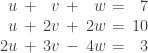
Exercise 1.3.9. State whether the following statements are true or false. (Note that without loss of generality we can assume that no row exchanges occur during the process of elimination.)

(a) Given a system in u, v, etc., where the third equation starts with zero (i.e., u has coefficient 0), during the process of elimination no multiple of the first equation will be subtracted from the third equation.

(b) Given a system in u, v, etc., where the third equation has zero as the second coefficient (i.e., v has coefficient 0), during the process of elimination no multiple of the second equation will be subtracted from the third equation.

(c) Given a system in u, v, etc., where the third equation has zero as both the first and the second coefficient (i.e., both u and v have coefficient 0), during the process of elimination no multiple of either the first or the second equation will be subtracted from the third equation.

Answer: (a) True. Since the coefficient of u in the third equation is already zero, in the first step of elimination there is no need to subtract a multiple of the first equation in order to transform the third equation into a new equation with a zero coefficient for u.

(b) False. Since the first coefficient (of u) of the third equation may be nonzero, in the first step of elimination we may need to subtract a multiple of the first equation from the third equation in order to transform the third equation into a new equation with a zero coefficient for u. In that case, if the second coefficient in the first equation is nonzero then that will result in the second coefficient (of v) in the third equation becoming nonzero.

In that event, in the next step of elimination we would need to subtract a multiple of the second equation from the third equation in order to transform the third equation into a new equation with a zero coefficient for v.

(c) True. As in (a), since the coefficient of u in the third equation is already zero, in the first step of elimination there is no need to subtract a multiple of the first equation in order to transform the third equation into a new equation with a zero coefficient for u. In that case the coefficient of v in the third equation would remain zero, and there would be no need to subtract a multiple of the second equation in order to transform the third equation into a new equation with a zero coefficient for v.

NOTE: This continues a series of posts containing worked out exercises from the (out of print) book Linear Algebra and Its Applications, Third Edition by Gilbert Strang.

If you find these posts useful I encourage you to also check out the more current Linear Algebra and Its Applications, Fourth Edition, Dr Strang’s introductory textbook Introduction to Linear Algebra, Fourth Edition and the accompanying free online course, and Dr Strang’s other books.

Posted in linear algebra | Leave a comment

Linear Algebra and Its Applications, exercise 1.3.8

Exercise 1.3.8. Given a system of equations of order n = 600, how long would it take to solve in terms of the number of multiplication-subtractions? In seconds, on a PC capable of 8,000 operations per second? On a VAX system capable of 80,000 operations per second? On a Cray X-MP/2 capable of 12 million operations per second?

Answer: As discussed in section 1.3, subsection The Cost of Elimination, for large n the number of operations is approximately \frac{1}{3}n^3. For n = 600 the number of operations is therefore approximately
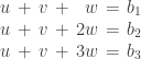
\frac{1}{3} \cdot 600^3 = \frac{1}{3} \cdot 6^3 \cdot 100^3 = \frac{1}{3} \cdot 2^3 \cdot 3^3 \cdot (10^2)^3 = 2^3 \cdot 3^2 \cdot 10^6 = 8 \cdot 9 \cdot 1,000,000 = 72,000,000

At 8,000 operations per second this would take 72,000,000 / 8,000 = 9,000 seconds (two and a half hours). At 80,000 operations per second this would take 900 seconds (15 minutes), At 12 million operations per second this would take six seconds.

NOTE: This continues a series of posts containing worked out exercises from the (out of print) book Linear Algebra and Its Applications, Third Edition by Gilbert Strang.

If you find these posts useful I encourage you to also check out the more current Linear Algebra and Its Applications, Fourth Edition, Dr Strang’s introductory textbook Introduction to Linear Algebra, Fourth Edition and the accompanying free online course, and Dr Strang’s other books.

Posted in linear algebra | Leave a comment

Linear Algebra and Its Applications, exercise 1.3.7

Exercise 1.3.7. (a) Given a system of equations A, with the first two rows the same, at what point in elimination will it become clear that A is singular? Show a 3×3 example.

(b) Repeat (a), but instead assume that the first two columns are the same.

Answer: (a) If the first two rows of A are the same then the first elimination step will produce zeros in the second row. The second step will do a row exchange in an attempt to get a non-zero pivot in the second row. Assuming that this is successful elimination will continue and can proceed as usual, doing row exchanges when necessary to avoid the problem of finding a zero in the pivot position due to the row of zeros. However at the point where the zero row is the last row row exchange can no longer correct the problem, and elimination will fail because there will not be a non-zero pivot.

The following example shows the process. We start with the system of equations

\setlength\arraycolsep{0.2em}\begin{array}{rcrcrcr}u&+&v&+&w&=&b_1       \\ u&+&v&+&w&=&b_2 \\ 2u&+&v&+&w&=&b_3 \end{array}

which in matrix form becomes

\left[ \begin{array}{rrrl} 1&1&1&b_1 \\ 1&1&1&b_2 \\ 2&1&1&b_3 \end{array} \right]

The first elimination step produces the following matrix

\left[ \begin{array}{rrrc} 1&1&1&b_1 \\ 0&0&0&b_2 - b_1 \\ 0&-1&-1&b_3 - 2b_1 \end{array} \right]

after which we can do a row exchange to produce

\left[ \begin{array}{rrrc} 1&1&1&b_1 \\ 0&-1&-1&b_3 - 2b_1 \\  0&0&0&b_2 - b_1 \end{array} \right]

However at this point we cannot find a nonzero pivot, elimination fails, and it is clear that the system of equations is singular.

(b) If the first two columns of A are identical, then the first elimination step will produce zeros not only in the first column of the second and subsequent rows, but zeros in the second column of the second and subsequent rows as well. There will therefore be no way that row exchange could produce a nonzero pivot in the second column of the second row, and at that point we will know that elimination has failed and the system of equations in singular.

\setlength\arraycolsep{0.2em}\begin{array}{rcrcrcr}u&+&v&+&w&=&b_1        \\ u&+&v&+&2w&=&b_2 \\ u&+&v&+&3w&=&b_3 \end{array}

which in matrix form becomes

\left[ \begin{array}{rrrl} 1&1&1&b_1 \\  1&1&2&b_2 \\ 1&1&3&b_3 \end{array} \right]

The first elimination step produces the matrix

\left[ \begin{array}{rrrc} 1&1&1&b_1 \\ 0&0&1&b_2 - b_1 \\ 0&0&2&b_3 - b_1 \end{array} \right]

which has no nonzero pivot in the second column, even allowing for row exchange.

NOTE: This continues a series of posts containing worked out exercises from the (out of print) book Linear Algebra and Its Applications, Third Edition by Gilbert Strang.

If you find these posts useful I encourage you to also check out the more current Linear Algebra and Its Applications, Fourth Edition, Dr Strang’s introductory textbook Introduction to Linear Algebra, Fourth Edition and the accompanying free online course, and Dr Strang’s other books.

Posted in linear algebra | Leave a comment