Linear Algebra and Its Applications, exercise 1.4.13

Exercise 1.4.13. Provide an example of multiplying two 3×3 triangular matrices, to confirm the general case that the product of triangular matrices is itself a triangular matrix. Prove the general case based on the definition of matrix multiplication.

Answer: An example of multiplying two 3×3 upper triangular matrices:

\begin{bmatrix} 1&1&1 \\ 0&1&1 \\ 0&0&1 \end{bmatrix} \begin{bmatrix} 1&2&3 \\ 0&1&2 \\ 0&0&1 \end{bmatrix} = \begin{bmatrix} 1&3&6 \\ 0&1&3 \\ 0&0&1 \end{bmatrix}

In general, for the two upper triangular matrices A and B, where A is mxn and B is nxp, we have

a_{ij} = 0, i > j and b_{ij} = 0, i > j

For the product C = AB we have

c_{ij} = \sum_{k=1}^{k=n} a_{ik}b_{kj} \: \rm for \: i = 1, \ldots, m \: \rm and \: j = 1, \ldots, p

Assume i > j. Then

1 \le k \le j \Rightarrow i > k \Rightarrow a_{ik} = 0 \Rightarrow a_{ik}b_{kj} = 0 \: \rm for \: k = 1, \ldots, j

and

j < k \le n \Rightarrow k > j \Rightarrow b_{kj} = 0 \Rightarrow a_{ik}b_{kj} = 0 \: \rm for \: k = j+1, \ldots, n

If i > j we thus have

a_{ik}b_{kj} = 0 \: \rm for \: k = 1, \ldots, n

But then if i > j we have

c_{ij} = \sum_{k=1}^{k=n} a_{ik}b_{kj} = \sum_{k=1}^{k=n} 0 = 0

Since c_{ij} = 0 for i > j, C = AB is an upper triangular matrix as well.

A similar argument shows that the product of two lower triangular matrices is also lower triangular. (For a lower triangular matrix A we would have a_{ij} = 0 if i < j.)

NOTE: This continues a series of posts containing worked out exercises from the (out of print) book Linear Algebra and Its Applications, Third Edition by Gilbert Strang.

If you find these posts useful I encourage you to also check out the more current Linear Algebra and Its Applications, Fourth Edition, Dr Strang’s introductory textbook Introduction to Linear Algebra, Fourth Edition and the accompanying free online course, and Dr Strang’s other books.

Posted in linear algebra | Leave a comment

Linear Algebra and Its Applications, exercise 1.4.12

Exercise 1.4.12. Given the matrices A and B below, the first row of their product AB is a linear combination of all the rows of B. Find the coefficients of this linear combination, and the first row of B.

A = \begin{bmatrix} 2&1&4 \\ 0&-1&1 \end{bmatrix} \quad B = \begin{bmatrix} 1&1 \\ 0&1 \\ 1&0  \end{bmatrix}

Answer: Since A is a 3×2 matrix and B is a 2×3 matrix, their product AB is a 2×2 matrix. In computing the first row of B we use the first row of A, with the three values 2, 1, and 4 respectively being the coefficients of the linear combination:

2 \cdot \begin{bmatrix} 1&1 \end{bmatrix} + 1 \cdot \begin{bmatrix} 0&1 \end{bmatrix} + 4 \cdot \begin{bmatrix} 1&0 \end{bmatrix} = \begin{bmatrix} 6&3 \end{bmatrix}

NOTE: This continues a series of posts containing worked out exercises from the (out of print) book Linear Algebra and Its Applications, Third Edition by Gilbert Strang.

If you find these posts useful I encourage you to also check out the more current Linear Algebra and Its Applications, Fourth Edition, Dr Strang’s introductory textbook Introduction to Linear Algebra, Fourth Edition and the accompanying free online course, and Dr Strang’s other books.

Posted in linear algebra | Leave a comment

Linear Algebra and Its Applications, exercise 1.4.11

Exercise 1.4.11. State whether the following statements are true or false. If a given statement is false, provide a counterexample to the statement.

  1. For two matrices A and B, if the first column of B is identical to the third column of B then the first column of AB is identical to the third column of AB.
  2. If the first row of B is identical to the third row of B then the first row of AB is identical to the third row of AB.
  3. If the first row of A is identical to the third row of A then the first row of AB is identical to the third row of AB.
  4. The square of AB is equal to the square of A times the square of B.

Answer: Assume that A is an m x n matrix and B is an n x p matrix.
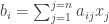
1. Each entry c_{i1} in the first column of AB is formed by taking the inner product of the ith row of A with the first column of B:
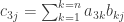
c_{i1} = \sum_{k=1}^{k=n} a_{ik}b_{k1}

Similarly, each entry c_{i3} in the third column of AB is formed by taking the inner product of the ith row of A with the third column of B:

c_{i3} = \sum_{k=1}^{k=n} a_{ik}b_{k3}

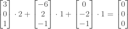
If the first column of B is equal to the third column of B then we have

b_{i1} = b_{i3} for all i = 1, \ldots, n

We then have

c_{i1} = \sum_{k=1}^{k=n} a_{ik}b_{k1} = \sum_{k=1}^{k=n} a_{ik}b_{k3} = c_{i3} \: \rm for \: i = 1, \ldots, m

so that the first column of AB is equal to the third column of AB. The statement is therefore true.

2. Each entry c_{1j} in the first row of AB is formed by taking the inner product of the first row of A with the jth column of B:

c_{1j} = \sum_{k=1}^{k=n} a_{1k}b_{kj}

Similarly, each entry c_{3j} in the third row of AB is formed by taking the inner product of the third row of A with the jth column of B:

c_{3j} = \sum_{k=1}^{k=n} a_{3k}b_{kj}

If the first and third rows of A are different then their inner products with each of the columns of B are not guaranteed to be equal in the general case, and thus the first and third rows of AB are not guaranteed to be equal in the general case. The statement is therefore false.

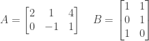
By making the first and third rows of B equal (as stated), but the first and third rows of A different, we can construct a suitable counterexample where the first and third rows of AB are different:

AB = \begin{bmatrix} 1&0&0 \\ 0&0&0 \\ 0&0&0 \end{bmatrix} \begin{bmatrix} 1&1&1 \\ 0&0&0 \\ 1&1&1  \end{bmatrix} = \begin{bmatrix} 1&1&1 \\ 0&0&0 \\ 0&0&0  \end{bmatrix}

3. As stated in the previous item, each entry c_{1j} in the first row of AB is formed by taking the inner product of the first row of A with the jth column of B:

c_{1j} = \sum_{k=1}^{k=n} a_{1k}b_{kj}

and each entry c_{3j} in the third row of AB is formed by taking the inner product of the third row of A with the jth column of B:

c_{3j} = \sum_{k=1}^{k=n} a_{3k}b_{kj}

If the first row of A is equal to the third row of A then their inner products with the jth column of B will be the same, and this implies in turn that each entry in the first row of AB will be equal to the corresponding entry in the third row of AB. The atatement is therefore true.

4. We can express the square of AB as follows:

(AB)^2 = (AB)(AB) = A(BA)B

using the definition of the square of AB and the associativity of matrix multiplication.

Similarly we can express the square of A times the square of B as:

A^2B^2 = (AA)(BB) = A(AB)B

Since matrix multiplication is not commutative AB \neq BA in the general case, which implies from the equations above that (AB)^2 \neq A^2B^2 in the general case. The statement is therefore false.

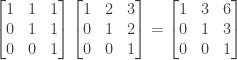
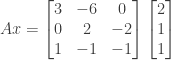
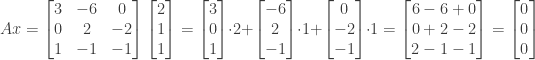
We can find a counterexample by finding two matrices A and B where AB \neq BA. For example, if

A = \begin{bmatrix} 1&1 \\ 0&1 \end{bmatrix} \: \rm and \: B = \begin{bmatrix} 1&0 \\ 1&1 \end{bmatrix}

we have

AB = \begin{bmatrix} 1&1 \\ 0&1 \end{bmatrix}  \begin{bmatrix} 1&0 \\ 1&1 \end{bmatrix} = \begin{bmatrix} 2&1 \\ 1&1 \end{bmatrix} \: \rm and \: BA = \begin{bmatrix} 1&0 \\ 1&1 \end{bmatrix}  \begin{bmatrix}  1&1 \\ 0&1 \end{bmatrix} = \begin{bmatrix} 1&1 \\ 1&2  \end{bmatrix}

A^2 = \begin{bmatrix} 1&1 \\ 0&1 \end{bmatrix} \begin{bmatrix} 1&1 \\ 0&1 \end{bmatrix} = \begin{bmatrix} 1&2 \\ 0&1 \end{bmatrix} \: \rm and \: B^2 = \begin{bmatrix} 1&0 \\ 1&1 \end{bmatrix} \begin{bmatrix} 1&0 \\ 1&1 \end{bmatrix} = \begin{bmatrix} 1&0 \\ 2&1 \end{bmatrix}

A^2B^2 = \begin{bmatrix} 1&2 \\ 0&1 \end{bmatrix}\begin{bmatrix} 1&0 \\ 2&1 \end{bmatrix} = \begin{bmatrix} 5&2 \\ 2&1 \end{bmatrix} \: \rm and \: (AB)^2 = \begin{bmatrix} 2&1 \\ 1&1 \end{bmatrix}  \begin{bmatrix} 2&1 \\ 1&1 \end{bmatrix} = \begin{bmatrix} 5&3 \\ 3&2 \end{bmatrix}

NOTE: This continues a series of posts containing worked out exercises from the (out of print) book Linear Algebra and Its Applications, Third Edition by Gilbert Strang.

If you find these posts useful I encourage you to also check out the more current Linear Algebra and Its Applications, Fourth Edition, Dr Strang’s introductory textbook Introduction to Linear Algebra, Fourth Edition and the accompanying free online course, and Dr Strang’s other books.

Posted in linear algebra | Leave a comment

Linear Algebra and Its Applications, exercise 1.4.10

Exercise 1.4.10. Given a matrix A with entries a_{ij}, what are the following entries?

  1. first pivot
  2. the multiplier l_{i1} that is used to multiply the first row and subtract it from the ith row
  3. the value that replaces a_{ij} once the above operation occurs
  4. second pivot

Answer: The first pivot is a_{11}, the entry in the first row and first column. (This assumes that that entry is non-zero and thus no row exchange is needed.)

For row i we need to eliminate the entry a_{i1}, the first entry in that row. Since l_{i1} is used to multiply the first row, we must have

a_{i1} - l_{i1}a_{11} = 0 \quad \Rightarrow \quad l_{i1}a_{11} = a_{i1} \quad \Rightarrow \quad l_{i1} = a_{i1}/a_{11}

Since l_{i1} is used to multiply all the entries in the first row and subtract the resulting value from corresponding entries in the ith row, the result of applying this operation to the entry a_{ij} is therefore

a_{ij} - l_{i1}a_{1j}

This operation is done on all rows, including the second row and the entry in the second column in that row, a_{22}. The resulting value

a_{22} - l_{21}a_{12}

then becomes the second pivot.

NOTE: This continues a series of posts containing worked out exercises from the (out of print) book Linear Algebra and Its Applications, Third Edition by Gilbert Strang.

If you find these posts useful I encourage you to also check out the more current Linear Algebra and Its Applications, Fourth Edition, Dr Strang’s introductory textbook Introduction to Linear Algebra, Fourth Edition and the accompanying free online course, and Dr Strang’s other books.

Posted in linear algebra | Leave a comment

Linear Algebra and Its Applications, exercise 1.4.9

Exercise 1.4.9. Given the following two examples of FORTRAN code

   DO 10 I=1,N
   DO 10 J=1,N
10 B(I) = B(I) + A(I,J)*X(J)

and

   DO 10 J=1,N
   DO 10 I=1,N
10 B(I) = B(I) + A(I,J)*X(J)

Do they multiply Ax by rows and columns?

Answer: The first code sample computes

b_i = \sum_{j=1}^{j=n} a_{ij} x_j

for a given i in the inner loop. Since i is constant for a_{ij} in the inner loop, the sum is for all entries in row i of A. The outer loop iterates over i, so the multiplication is done by rows.

The second code sample holds j constant in the inner loop and iterates over the entries of A in column j. The outer loop iterates over j, so the second sample is multiplying by columns.

NOTE: This continues a series of posts containing worked out exercises from the (out of print) book Linear Algebra and Its Applications, Third Edition by Gilbert Strang.

If you find these posts useful I encourage you to also check out the more current Linear Algebra and Its Applications, Fourth Edition, Dr Strang’s introductory textbook Introduction to Linear Algebra, Fourth Edition and the accompanying free online course, and Dr Strang’s other books.

Posted in linear algebra | Leave a comment

Linear Algebra and Its Applications, exercise 1.4.8

Exercise 1.4.8. Give non-zero examples of 3×3 matrices with the following properties:

  1. diagonal matrix (a_{ij} = 0 if i \neq j);
  2. symmetric matrix (a_{ij} = a_{ji} for all i \neq j);
  3. upper triangular matrix (a_{ij} = 0 if i > j);
  4. skew-symmetric matrix (a_{ij} = -a_{ji} for all i and j).

Answer: Diagonal matrix:

\begin{bmatrix} 1&0&0 \\ 0&2&0 \\ 0&0&3 \end{bmatrix}

Symmetric matrix:

\begin{bmatrix} 1&2&3 \\ 2&2&4 \\ 3&4&3 \end{bmatrix}

Upper triangular matrix:

\begin{bmatrix} 1&2&3 \\ 0&2&3 \\ 0&0&3 \end{bmatrix}

Skew-symmetric matrix:

\begin{bmatrix} 0&2&3 \\ -2&0&4 \\  -3&-4&0 \end{bmatrix}

NOTE: This continues a series of posts containing worked out exercises from the (out of print) book Linear Algebra and Its Applications, Third Edition by Gilbert Strang.

If you find these posts useful I encourage you to also check out the more current Linear Algebra and Its Applications, Fourth Edition, Dr Strang’s introductory textbook Introduction to Linear Algebra, Fourth Edition and the accompanying free online course, and Dr Strang’s other books.

Posted in linear algebra | Leave a comment

Linear Algebra and Its Applications, exercise 1.4.7

Exercise 1.4.7. Given the n-dimensional row vector y and column vector x, express their inner product in summation notation.

Answer: We have

yx = \begin{bmatrix} y_1&y_2&\cdots&y_n \end{bmatrix} \begin{bmatrix} x_1 \\ x_2 \\ \vdots \\ x_n \end{bmatrix} = y_1 x_1 + y_2 x_2 + \cdots + y_n x_n = \sum_{i = 1}^{i = n} y_i x_i

NOTE: This continues a series of posts containing worked out exercises from the (out of print) book Linear Algebra and Its Applications, Third Edition by Gilbert Strang.

If you find these posts useful I encourage you to also check out the more current Linear Algebra and Its Applications, Fourth Edition, Dr Strang’s introductory textbook Introduction to Linear Algebra, Fourth Edition and the accompanying free online course, and Dr Strang’s other books.

Posted in linear algebra | Leave a comment

Linear Algebra and Its Applications, exercise 1.4.6

Exercise 1.4.6. Find the 3×2 matrix A for which a_{ij} = i + j
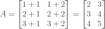
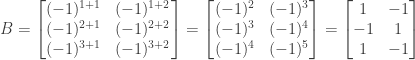
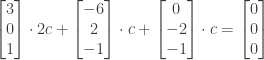
. Find the 3×2 matrix B for which b_{ij} = (-1)^{i+j}.

Answer: We have

A = \begin{bmatrix} 1+1&1+2 \\ 2+1&2+2 \\ 3+1&3+2 \end{bmatrix} = \begin{bmatrix} 2&3 \\ 3&4  \\ 4&5 \end{bmatrix}

We also have

B = \begin{bmatrix} (-1)^{1+1}&(-1)^{1+2} \\ (-1)^{2+1}&(-1)^{2+2}  \\ (-1)^{3+1}&(-1)^{3+2}\end{bmatrix} = \begin{bmatrix} (-1)^2&(-1)^3 \\ (-1)^3&(-1)^4 \\ (-1)^4&(-1)^5 \end{bmatrix} = \begin{bmatrix} 1&-1 \\ -1&1 \\ 1&-1 \end{bmatrix}

NOTE: This continues a series of posts containing worked out exercises from the (out of print) book Linear Algebra and Its Applications, Third Edition by Gilbert Strang.

If you find these posts useful I encourage you to also check out the more current Linear Algebra and Its Applications, Fourth Edition, Dr Strang’s introductory textbook Introduction to Linear Algebra, Fourth Edition and the accompanying free online course, and Dr Strang’s other books.

Posted in linear algebra | Leave a comment

Linear Algebra and Its Applications, exercise 1.4.5

Exercise 1.4.5. Multiply the following matrices:

Ax = \begin{bmatrix} 3&-6&0 \\ 0&2&-2 \\ 1&-1&-1 \end{bmatrix}  \begin{bmatrix} 2  \\ 1 \\ 1 \end{bmatrix}

Considering the matrix A as a system of equations, find a solution to the system Ax = 0, for which the right-hand side of all three equations is zero. Specify whether there is just one solution or many; if the latter find another solution.

Answer:Working by columns we have

Ax = \begin{bmatrix} 3&-6&0 \\ 0&2&-2 \\  1&-1&-1 \end{bmatrix}  \begin{bmatrix} 2  \\ 1 \\ 1  \end{bmatrix} = \begin{bmatrix} 3 \\ 0 \\ 1 \end{bmatrix} \cdot 2 + \begin{bmatrix} -6 \\ 2 \\ -1 \end{bmatrix} \cdot 1 + \begin{bmatrix} 0 \\ -2 \\ -1 \end{bmatrix} \cdot 1 = \begin{bmatrix} 6 - 6 + 0 \\ 0 + 2 - 2 \\ 2 - 1 - 1 \end{bmatrix} = \begin{bmatrix} 0 \\ 0 \\ 0 \end{bmatrix}

So we have (2, 1, 1) as a solution vector to the system of equations.

Going back to the equation

\begin{bmatrix} 3 \\ 0 \\ 1 \end{bmatrix} \cdot 2 +  \begin{bmatrix} -6 \\ 2 \\ -1 \end{bmatrix} \cdot 1 + \begin{bmatrix} 0  \\ -2 \\ -1 \end{bmatrix} \cdot 1 = \begin{bmatrix} 0 \\ 0 \\ 0  \end{bmatrix}

we see that we can multiply both sides of the equation by a constant c:

\begin{bmatrix} 3 \\ 0 \\ 1 \end{bmatrix} \cdot 2c +   \begin{bmatrix} -6 \\ 2 \\ -1 \end{bmatrix} \cdot c + \begin{bmatrix} 0   \\ -2 \\ -1 \end{bmatrix} \cdot c = \begin{bmatrix} 0 \\ 0 \\ 0   \end{bmatrix}

So (2c, c, c) is also a solution for any c; for c = 2 we have the solution (4, 2, 2).

NOTE: This continues a series of posts containing worked out exercises from the (out of print) book Linear Algebra and Its Applications, Third Edition by Gilbert Strang.

If you find these posts useful I encourage you to also check out the more current Linear Algebra and Its Applications, Fourth Edition, Dr Strang’s introductory textbook Introduction to Linear Algebra, Fourth Edition and the accompanying free online course, and Dr Strang’s other books.

Posted in linear algebra | Leave a comment

Linear Algebra and Its Applications, exercise 1.4.4

Exercise 1.4.4. Compute the number of multiplications required to multiply an mxn matrix A by an n-dimensional vector x. Also compute the number of multiplications required to multiply A by an nxp matrix B.

Answer: The result of multiplying A (which is mxn) by x (which is nx1) is an mx1 column vector b. Each entry of b is the inner product of a row of A (containing n entries) with all the n entries of x, and therefore requires n multiplications. Since b has m entries, the total number of multiplications is thus m times n or mn.

More formally, for each entry b_i of b we have

b_i = \sum_{j = 1}^{j = n} a_{ij}x_j, \: { \rm for } \: i = 1, \ldots, m

Each sum requires n multiplications, and there are m sums in toto.

When multiplying A times B, the result is the mxp matrix AB. Each entry of AB is the inner product of a row of A (containing n entries) and a column of B (also containing n entries), and requires n multiplications. Since AB contains m times p entries, the total number of multiplications is therefore m times p times n or mnp.

More formally, for each entry c_{ij} of B we have

c_{ij} = \sum_{k = 1}^{k = n} a_{ik}b_{kj}, \: { \rm for } \: i = 1,  \ldots, m \: { \rm and } \: j = 1, \ldots, p

Each sum requires n multiplications, and there are m times p sums in toto.

NOTE: This continues a series of posts containing worked out exercises from the (out of print) book Linear Algebra and Its Applications, Third Edition by Gilbert Strang.

If you find these posts useful I encourage you to also check out the more current Linear Algebra and Its Applications, Fourth Edition, Dr Strang’s introductory textbook Introduction to Linear Algebra, Fourth Edition and the accompanying free online course, and Dr Strang’s other books.

Posted in linear algebra | 1 Comment