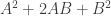
Exercise 1.4.14. Show example 2×2 matrices having the following properties:
- A matrix A with real entries such that

- A nonzero matrix B such that

- Two matrices C and D with nonzero product such that CD = -DC
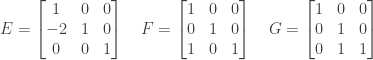
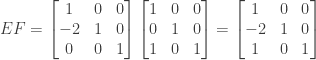
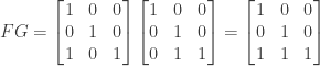
- Two matrices E and F with all nonzero entries such that EF = 0
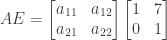
Answer: (a) If we have
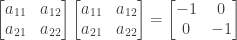
We then have the following:


Assume that  . From the first and fourth equations above we then have


which reduces to the single equation  . Assume that
  for some real nonzero a. We then have
  .
.
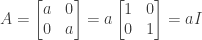
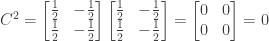
So a matrix A meeting the above criterion is

where a is nonzero, for which

We can obtain a specific example of A by setting a = 1, in which case

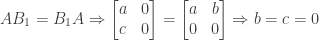
(b) If we have

We then have the following:


Assume that  and
and  are nonzero, and choose
  where b is a nonzero real number. Then from the second and third equations we have
  . From the first and fourth equations we should have
  and this is indeed the case, since
  .
.
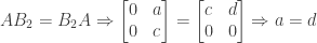
Substituting into the first equation we then have

(We could have used the fourth equation just as well for this.)
If we choose  we then have
  . This gives us the following matrix

for which

If we set b = 1 then we obtain the specific example

(c) If  we have

By the rules of matrix multiplication we then have


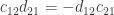
Taking the second and third equations above and rearranging terms we have


The easiest way to satisfy the resulting equations is to set

We then have

which gives us the following equations:

which reduce to the single equation  . If we set
  where
where  then we have
  . If we set
  where
where  then
then  . We then have the following matrices C and D:

with
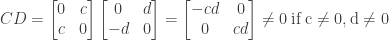
and

One example of C and D can be found by setting  :
:

(d) Using the result of (b) above, if we set

then we will have EF = 0 with both E and F having all nonzero entries.
NOTE: This continues a series of posts containing worked out exercises from the (out of print) book Linear Algebra and Its Applications, Third Edition by Gilbert Strang.
If you find these posts useful I encourage you to also check out the more current Linear Algebra and Its Applications, Fourth Edition , Dr Strang’s introductory textbook Introduction to Linear Algebra, Fourth Edition
 and the accompanying free online course, and Dr Strang’s other books
 .
.


 by the following matrix:
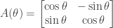
 . Hint: use the identities for
  and
and  .
. .
.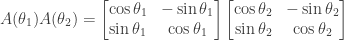


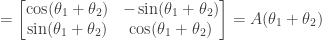
 as hypothesized. In other words, rotating the x-y plane through an angle
  followed by a second rotation through an angle
  is equivalent to a single rotation through the angle
  .
.
 (i.e., through the angle
 is the ith column of A,
  is the ith row of B, and the product
  is a matrix.
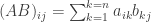


 . If we define
  then we have
 of their product AB? Use the following summation formula to find the answer:
 for all i and j, then we have
 for all i and j, then the i-jth entry of (AB)C is

 ?
?