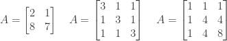
Exercise 1.4.24. The following matrices can be multiplied using block multiplication, with the indicated submatrices within the matrices multiplied together:

- Provide example matrices matching the templates above and use block multiplication to multiply them together.
- Provide two example templates for multiplying a 3×4 matrix A and 4×2 matrix B using block multiplication.
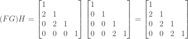
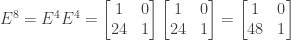
Answer: (a) For the first example we multiply the following matrices using block multiplication on the indicated submatrices:

To do block multiplication we must multiply all submatrices that are capable of being multiplied, i.e., the number of columns in the first submatrix is equal to the number of columns rows in the second submatrix. We then take the product of each pair of submatrices, assign it a spot in the final product matrix, and sum the resulting matrices to get the answer.
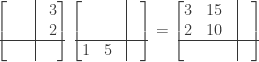
In the above example we start by multiplying the upper left 2×2 submatrix in the first matrix with the upper left 2×2 submatrix in the second matrix:

and then with the upper right 2×1 submatrix in the second matrix:

We next multiply the 2×1 upper right submatrix in the first matrix with the 1×2 lower left submatrix in the second matrix:
and then with the 1×1 lower right submatrix in the second matrix:
We next multiply the lower left 1×2 submatrix in the first matrix with the upper left 2×2 submatrix in the second matrix:

and then with the upper right 2×1 submatrix in the second matrix:

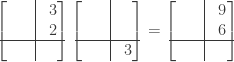
Finally we multiple the 1×1 submatrix in the lower right of the first matrix with the 1×2 submatrix in the lower left of the second matrix:

and with the 1×1 submatrix in the lower right of the second matrix:

Then we add all of the resulting matrices together:


and compare to the result of conventional matrix multiplication:

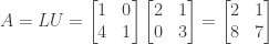
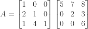
For the second example we multiply the following matrices using block multiplication on the indicated submatrices:

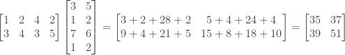
We start by multiplying the left 2×2 submatrix in the first matrix with the upper 2×2 submatrix in the second matrix:

and then multiply the right 2×2 submatrix in the first matrix with the lower 2×2 submatrix in the second matrix:

Then we add the two resulting matrices together:

and compare to the result of conventional matrix multiplication:
(b) In multiplying a 3×4 matrix by a 4×2 matrix using block multiplication, one possible way to divide the matrices is as follows:

This results in multiplying the left 3×2 submatrix of the first matrix by the upper 2×2 submatrix of the second matrix to produce a 3×2 matrix, and multiplying the right 3×2 submatrix of the first matrix by the lower 2×2 submatrix of the second matrix to produce a second 3×2 matrix. The two 3×2 matrices are then added to produce the final 3×2 product matrix.
Another slightly more complicated approach is as follows:

This results in multiplying the left 3×3 submatrix of the first matrix by the upper 3×2 submatrix of the second matrix to produce a 3×2 matrix, and multiplying the right 3×1 submatrix of the first matrix by the lower 1×2 submatrix of the second matrix to produce a second 3×2 matrix. The two 3×2 matrices are then added to produce the final 3×2 product matrix.
NOTE: This continues a series of posts containing worked out exercises from the (out of print) book Linear Algebra and Its Applications, Third Edition by Gilbert Strang.
If you find these posts useful I encourage you to also check out the more current Linear Algebra and Its Applications, Fourth Edition , Dr Strang’s introductory textbook Introduction to Linear Algebra, Fourth Edition
 and the accompanying free online course, and Dr Strang’s other books
 .
.

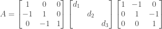


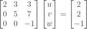
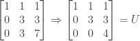
 times row 1 of U and
  times row 2 of U. (Note that for simplicity we assume that no row exchanges are necessary.)
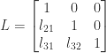


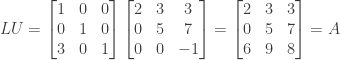
 where
where
 where
where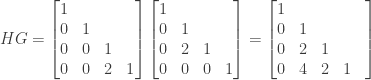

 .
.
 ,
,  , and
, and  .
.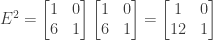
 or 12. If we change the second 6 to -6 we instead obtain
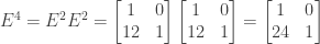
  or zero for the 2,1 position. We then have
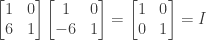


 is the identity matrix I.
 is also the identity matrix I.


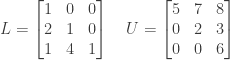
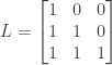
 are the entries below the diagonal of L, with
  for all i, j.
