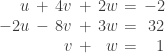
Exercise 1.5.14. Find all possible 3 by 3 permutation matrices, along with their inverses.
Answer: The identity matrix I is the first possible permutation matrix, corresponding to not doing a row exchange at all; it is its own inverse:


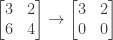
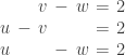
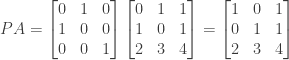
The permutation matrix  exchanges rows 1 and 2:
A second exchange of rows 1 and 2 returns both rows to their original position, so is its own inverse:
The permutation matrix  exchanges rows 1 and 3:

A second exchange of rows 1 and 3 returns both rows to their original position, so is also its own inverse:

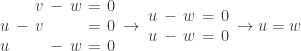
The permutation matrix  exchanges rows 2 and 3:

As with and (and for similar reasons) is also its own inverse:

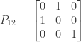
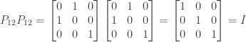
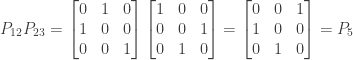
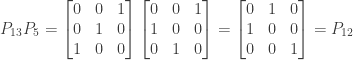
We can generate a fifth permutation matrix by exchanging rows 1 and 3 and then exchanging rows 2 and 3; this is equivalent to multiplying by :

(Note that the order of multiplication is important here; since by convention we apply permutation matrices to the left, we put on the right and then multiply it by on the left.) The resulting matrix sends row 1 to row 2, row 2 to row 3, and row 3 to row 1.
We can generate a sixth permutation matrix by reversing the exchanges used in creating the previous permutation matrix; in other words, we first exchange rows 2 and 3, and then subsequently exchange rows 1 and 3. This is equivalent to multiplying by :

The resulting matrix sends row 1 to row 3, row 2 to row 1, and row 3 to row 2, reversing the effect of the fifth permutation matrix. The fifth and sixth matrices are therefore inverses of each other:


In permuting the rows of a 3 by 3 matrix, we have three possible choices for row 1 of the permuted matrix. (In other words, row 1 of the permuted matrix could be set to row 1, row 2, or row 3 of the original matrix.) Having made that choice, we have two choices remaining for row 2 of the permuted matrix. (For example, if we set row 1 of the permuted matrix to be row 3 of the original matrix, then row 2 of the permuted matrix could be set to either row 1 or row 2 of the original matrix.)
Having made the first two choices, there is only one choice remaining for row 3 of the permuted matrix. (For example, if we set row 1 of the permuted matrix to be row 3 of the original matrix and row 2 of the permuted matrix to be row 1 of the original matrix, then row 3 of the permuted matrix must be set to row 2 of the original matrix.) There are thus 3 times 2 times 1 or 6 possible ways to permute the rows of a 3 x 3 matrix. (This is a special case of the general result that there are n times n-1 times n-2 … times 2 times 1 or  ways to permute n items.)
We have found six 3 by 3 permutation matrices:


This therefore completes the set of all possible 3 x 3 permutation matrices.
Extra credit: From above we have six 3 by 3 permutation matrices: I, , , ,  (equal to
  ), and
  (equal to
  ). There are 36 possible products of the six matrices (six possible choices for the left factor, and six for the right). We already know that IA = AI = A for any matrix A. We also know that any of , , and times itself equals I, since each of these three matrices is its own inverse. Finally, we know that equals , equals , and
  equals
  equals I.
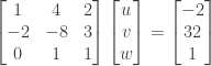
What about other products? We have

and

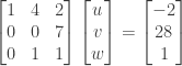
We also have
and

We then have

and

We next find the products of and with , , and respectively. We start by multiplying by on the left:


and then on the right:

We can then use the results above to compute products involving by taking advantage of the fact that is the inverse of :


Finally, we multiply and by themselves:


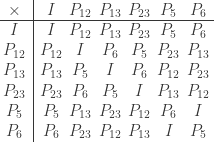
So the product of any two of the six 3 x 3 permutation matrices is itself one of the six permutation matrices. The following multiplication table summarizes the results above:
NOTE: This continues a series of posts containing worked out exercises from the (out of print) book Linear Algebra and Its Applications, Third Edition by Gilbert Strang.
If you find these posts useful I encourage you to also check out the more current Linear Algebra and Its Applications, Fourth Edition , Dr Strang’s introductory textbook Introduction to Linear Algebra, Fourth Edition
 and the accompanying free online course, and Dr Strang’s other books
 .
.


 and
and  and
and 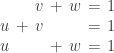


 and
and 


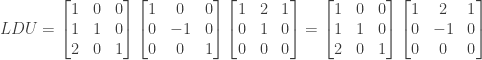


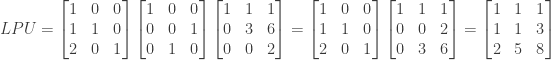
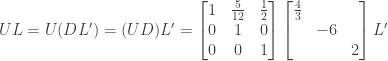
 be factored into the product
  where
where  is upper triangular and
  is lower triangular, instead of being factored into the product
  ? If so, how could this other factorization be carried out? Would
  of
of  ,
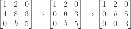
,  , and so on, up to row 1, and trying to produce zeros starting from column
  ; a multiple of row
  ; and so on. This produces a lower triangular matrix.

 times row 3 from row 1, and put the multiplier
 times row 2 from row 1, and put the multiplier

 . Note that if we reverse the order of the factors we have
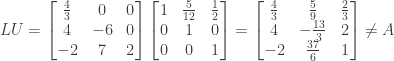
 , or vice versa—and indeed we would not expect this in general, since matrix multiplication is not commutative.
 times a new lower triangular matrix. We can then multiply the matrix


 is another factoring of
  is no longer a factoring:


 multiplication-substraction steps to solve. Explain why.
 can be found in a single operation, while solving for
  takes two operations, solving for
  three operations, and so on until solving for
  takes n operations.

 takes one step, solving for
  two steps, and so on until solving for
  takes n steps. Again the total number of steps is
  .
. steps for large n. As a result of performing elimination on A we obtain its two factors L and U. Given the particular system Ax = b we can use Lc = b to solve for c in approximately
  steps in all.


