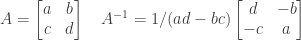
Exercise 1.6.2. (a) Find the inverses of the following matrices:

(b) Why does  for any permutation matrix P?
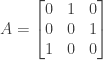
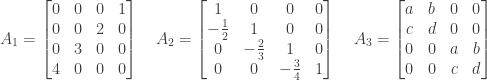
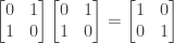
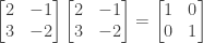
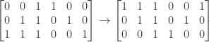
Answer: (a) The first permutation matrix exchanges the first and third rows of the identity matrix I, while leaving the second row the same. If we apply the permutation matrix again then the first and third rows will be exchanged back into their former positions, and the resulting matrix will be the identity matrix again:

So we have
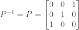
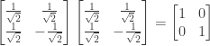
For the second matrix, we note that for the (1, 1) entry of the product of P and its inverse to be equal to one (as it would be if the product were the identity matrix), we must multiply the (1, 3) entry of P by one, which implies that the (3, 1) entry of the inverse is one, since we are multiplying the first row of P by the first column of its inverse.
Similarly, for the (2, 2) entry of the product to be one, we must multiply the (2, 1) entry of P by one, which implies that the (1, 2) entry of the inverse is one, since we are multiplying the second row of P by the second column of its inverse.
Finally, for the (3, 3) entry of the product to be one, the (3, 2) entry of P must multiply an entry of one in the (2,3) position of the inverse.
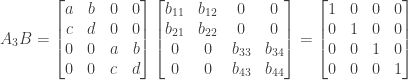
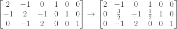
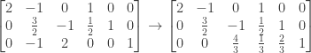
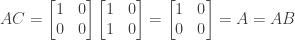
Constructing the matrix A where
we then have

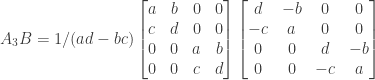
and

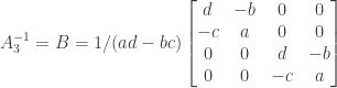
so that

(b) A permutation matrix P permutes the rows of a matrix it multiples (on the left). Multiplying the identity matrix I by P (on the left) thus permutes the rows of I, and since PI = P, P itself is a permutation of the rows of I.
Now consider the matrix A consisting of P multiplied by the transpose of P. The (i, j) entry of A is found by multiplying row i of P by column j of its transpose. But column j of P’s transpose is simply row j of P, so the (i, j) entry of A equals row i of P times row j of P.
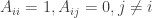
Each row of the identity matrix I contains a one in some column, with that column being different for each row. Since P is a permutation of I, this is true for P as well. So when i = j the (i, j) entry of A is the product of row i of P with itself, which in turn is a sum where all terms but one consist of zero multiplying zero, and the remaining term consists of one multiplying one. When i = j the (i, j) entry of A is therefore one.
On the other hand, when i does not equal j the (i, j) entry of A is the product of row i of P with a different row j of P. Since the two rows will have a one in different columns, this product is a sum where every term is either zero multiplying zero, zero multiplying one, or one multiplying zero. For non-equal i and j the (i, j) entry of A is therefore zero.
Since A has all zero entries except on the diagonal where i = j, A is the identity matrix and we have

Now consider the matrix B produced by multiplying the transpose of P times P. The (i, j) entry of B is the product of row i of the transpose of P times column j of P, which in turn is simply column i of P times column j of P.
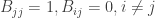
Each column of the identity matrix I contains a one in some row, with that row being different for each column. Since P is simply a permutation of the rows of I, this is true for P as well. So when i = j the (i, j) entry of B is the product of column i of P with itself, which in turn is a sum where all terms but one consist of zero multiplying zero, and the remaining term consists of one multiplying one. When i = j the (i, j) entry of B is therefore one.
On the other hand, when i does not equal j the (i, j) entry of B is the product of column i of P with a different column of P. Since the two columns will have a one in different rows, this product is a sum where every term is either zero multiplying zero, zero multiplying one, or one multiplying zero. For non-equal i and j the (i, j) entry of B is therefore zero.
Since B has all zero entries except on the diagonal where i = j, B is the identity matrix and we have
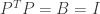
Since the transpose of P is both a left inverse of P and a right inverse of P, the transpose of P is the (unique) inverse of P.
Here is a more formal proof: Since P is a permutation of the identity matrix I, for each row i of P there is a k for which

and

Consider the matrix A where

We then have

For  we have


Since for each row i we have
A is the identity matrix I and we have
.
Since P is a permutation of the identity matrix I, for each column j of P there is a k (which may be different from the one above) for which

and

Consider the matrix B where

We then have

For  we have


Since for each column j we have
B is the identity matrix I and we have
.
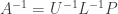
Since the transpose of P is both a left and right inverse of P it is the unique inverse of P, and we have
for every permutation matrix P.
NOTE: This continues a series of posts containing worked out exercises from the (out of print) book Linear Algebra and Its Applications, Third Edition by Gilbert Strang.
If you find these posts useful I encourage you to also check out the more current Linear Algebra and Its Applications, Fourth Edition , Dr Strang’s introductory textbook Introduction to Linear Algebra, Fourth Edition
 and the accompanying free online course, and Dr Strang’s other books
 .
.


 by the columns of A should give the third row of I. Explain why this is not possible.


 is invertible and has inverse B. Prove that A is also invertible, with inverse AB.


 .
.


 in the formula for
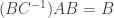
 was a left inverse for A.)