Exercise 1.6.12. Suppose that A is an invertible matrix and has one of the following properties:
(1) A is a triangular matrix.
(2) A is a symmetric matrix.
(3) A is a tridiagonal matrix.
(4) All the entries of A are whole numbers.
(5) All the entries of A are rational numbers (i.e., fractions or whole numbers).
Which of the above would also be true of the inverse of A? Prove your conclusions or find a counterexample if false.
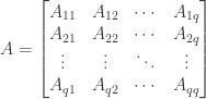
Answer: (1) Assume that A is an invertible triangular matrix. A can be either upper triangular or lower triangular. We first assume that A is upper triangular, such that

We use Gauss-Jordan elimination to find the inverse of A. Since A is upper triangular forward elimination is complete, since all entries beneath the diagonal of A are already zero. (Moreover, the diagonal entries of A are nonzero, since if there were any zeros in the pivot position A would be singular and hence not invertible.)
We can thus proceed immediately to backward elimination. The first backward elimination step multiplies all entries in the last row and subtracts them from the next-to-last row. But we still have I on the righthand side, and I has all zero entries below the diagonal just as A does. We will be multiplying zero entries below the diagonal of the right-hand matrix (i.e., in the last row), and then subtracting the resulting zero values from other zero values below the diagonal of the right-hand side (i.e., in the next to last row). As a result, after the first backward elimination step all the entries below the diagonal of the right-hand matrix will still be zero.
By similar reasoning the second step of backward elimination will also produce zero entries below the diagonal of the right-hand matrix, and so will each subsequent step. When Gauss-Jordan backward elimination finally completes, the final right-hand matrix, which is the inverse of A, will thus have all zero entries below the diagonal and will be upper triangular. Thus if A is upper triangular and invertible then the inverse of A will be upper triangular as well.
Now suppose A is invertible and lower triangular, so that

Again we do Gauss-Jordan elimination to find the inverse of A. The first forward elimination step multiplies all entries in the first row and subtracts them from the second row. We will be multiplying zero entries above the diagonal of both the left-hand and the right-hand matrix (i.e., in the first row), and then subtracting the resulting zero values from other zero values above the diagonal of the left-hand and the right-hand matrix (i.e., in the second row). As a result, after the first forward elimination step all the entries above the diagonal of both the left-hand and the right-hand matrix will still be zero.
By similar reasoning the second step of forward elimination will also produce zero entries above the diagonal of both the left-hand and right-hand matrix, and so will each subsequent step. After forward elimination completes both the lefthand matrix and the righthand matrix will thus have zeroes above the diagonal. Since the lefthand matrix has all zeroes above the diagonals there is no need to do backward elimination, and all that remains is to divide both matrices by the values in the pivot positions.
This division will leave any zero entries still zero, so the final righthand matrix, i.e., the inverse of A, will also have zeroes above the diagonal and will be lower triangular. Thus if A is lower triangular and invertible then the inverse of A will be lower triangular as well. Combining these two results, if A is an invertible triangular matrix then the inverse of A is triangular as well.
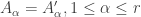
(2) Suppose that A is an invertible symmetric matrix. Since A is symmetric we have

and since A is invertible we have
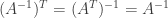
But since the inverse of A is equal to its own transpose it is a symmetric matrix. Thus if A is an invertible symmetric matrix then the inverse of A is also symmetric.
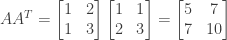
(3) We attempt to find a counter-example by constructing a 4 by 4 tridiagonal matrix A such that:
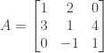
and then use Gauss-Jordan elimination to find its inverse:

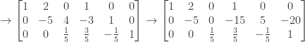
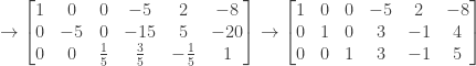
We therefore have

which is not a tridiagonal matrix. Therefore if A is an invertible tridiagonal matrix it is not necessarily the case that the inverse of A is also tridiagonal.
(4) We attempt to find a counter-example by constructing a 2 by 2 matrix A with whole number entries:

We then have

which does not have whole number entries. Therefore if A is an invertible matrix whose entries are all whole numbers, it is not necessarily the case that all the entries of the inverse of A are also whole numbers.
(5) Suppose that A is an invertible matrix and that all of the entries of A are rational numbers (whole numbers or fractions). For each i and j the corresponding entry of A is thus of the form

where p is some integer and q is some non-zero integer. (If q is 1 then the entry is a whole number.)
We use Gauss-Jordan elimination to find the inverse of A, and without loss of generality assume that no row exchanges are required for the first step. The first forward elimination step multiplies all entries in the first row and subtracts the results from each of the remaining rows, with the multipliers for each row being computed as the pivot in the first row divided by each of the entries in the same column of the remaining rows (assuming those entries are nonzero).
But a rational number divided by a nonzero rational number is itself a rational number, as is a rational number multiplied by another rational number, and as is a rational number added to or subtracted from another rational numbers. (See below for the proof of this.) Since all the entries in A are rational numbers, as are all in the entries in I (the right-hand matrix for the first elimination step), all the entries in the left-hand and right-hand matrices resulting from the first forward elimination step are also rational numbers.
By similar reasoning the second forward elimination step will produce only rational numbers, as will any subsequent elimination step. Similarly backward elimination will produce only rational numbers at each step, as will the final division by the nonzero pivots. The right-hand matrix after the final step, i.e., the inverse of A, thus has all entries being rational numbers. So if A is an invertible matrix with all rational entries then the inverse of A will also have all rational entries.
Proof that the product, sum, and difference of two rational numbers are themselves rational numbers, as is the result of dividing a rational number by a nonzero rational number:
Let a and b be rational numbers. We then have

for some p, q, r, and s where p and r are integers and q and s are nonzero integers.
The product of a and b is then

Since p and q are both integers their product is an integer, and since r and s are both nonzero integers their product is also a nonzero integer. The product of a and b can thus be expressed as an integer divided by a nonzero integer, and thus is a rational number.
The sum of a and b is then

The product of p and s is an integer, as is the product of q and r, and thus their sum is an integer as well. Also, since q and s are nonzero integers their product is a nonzero integer as well. The sum of a and b can thus be expressed as an integer divided by a nonzero integer, and thus is a rational number.
The difference of a and b can be show to be a rational number by a similar argument.
Finally, if b is nonzero then a divided by b is

Since p and s are integers their product is an integer as well. We also have q as a nonzero integer and since b is nonzero r is also a nonzero integer, so that the product of q and r is a nonzero integer as well. The result of dividing a by b can thus be expressed as an integer divided by a nonzero integer, and thus is a rational number.
NOTE: This continues a series of posts containing worked out exercises from the (out of print) book Linear Algebra and Its Applications, Third Edition by Gilbert Strang.
If you find these posts useful I encourage you to also check out the more current Linear Algebra and Its Applications, Fourth Edition , Dr Strang’s introductory textbook Introduction to Linear Algebra, Fourth Edition
 and the accompanying free online course, and Dr Strang’s other books
 .
.


 is a diagonal matrix and D is also a diagonal matrix, the product
  must also be a diagonal matrix. If it were not, and had at least one entry
 and
and  have ones on the diagonal. Since
  and
and  have entries
  . Since
  , for the (i, i) entry of
  we therefore have


 are upper triangular matrices with ones on the diagonal, their product


 can be factored as shown above, we have
 entries. We can select n independent entries to go on the diagonal, leaving
  off-diagonal entries to be chosen. However since A is a symmetric matrix only half of those entries (e.g., those above the diagonal) can be chosen independently, since the corresponding entries in the other part of the matrix (in this case, below the diagonal) will be the same.
 we must have
  for all
  , so that all the entries on the diagonal must be zero. Since the entries on the diagonal cannot be chosen independently, the number of independent entries is just half the number of off-diagonal entries, or


 . For all elements of A we then have


 and
and  are symmetric matrices. Provide an example where these matrices are not equal.
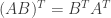


 ,
,  ,
,  , and
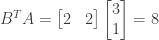
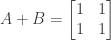
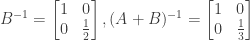
, and  for the following matrices:
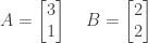


 is also invertible, and find an expression for its inverse. Hint: use the fact that


 be an
be an  by
by  matrix and a

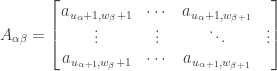
 can be described as a block matrix with
 . The partition is done using a vector
  of nonnegative integer values defined as follows:
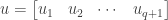


 is the first row in the
  partition,
  is the last row in the
  is the number of rows in the
  , using a vector
  of nonnegative integer values defined as follows:
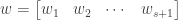


 is the first column in the
  is the last column in the
  is the number of columns in the
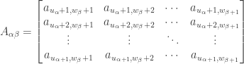
 entry of
  has the value
 we have


 and
and  we have


 of nonnegative integer values defined as follows:

 is the first column in the
  is the last column in the
  is the number of columns in the
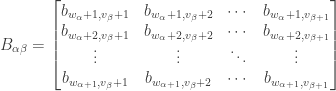
 then there is only a single submatrix of
  then each submatrix contains a single entry of
  has the value

 into
into 
 having the value
 and
and  where
where  and
and  .
. have
have  rows and
  columns, and all the submatrices
  have
have  columns. (This follows from the definitions of
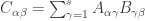
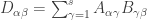
  is the sum of the product matrices, it too will have


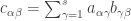
 ) starts at
  (because
  by definition), that each subsequent inner sum starts at a value of
  one greater than the last, and that the last inner sum (when
  ) ends at
  (because
  ). We thus conclude that
 , we conclude that
  , and from the definition of
  that
that then
then


 instead of
  for
for  , because I think it better corresponds to the intuitive idea of how a partition would be defined.
 and we have
  with
with  . Let
. Let  . We have
  when
when  . We have
  based on the new condition (assuming that
  so that
  has a value), so
  .
. has a value. Since
  and
and  has a value (since
  does) we then have
  . Thus
  and
and  , the old condition that
