
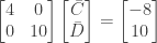
Exercise 3.4.6. Given the matrix
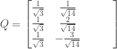
find entries for the third column such that 
Answer: In order for

so that the entry itself would be 
Similarly the square of the last entry of the second row must be

so that the entry itself would be 
Finally, the square of the last entry of the third row must be

so that the entry itself would be 
We have two possible choices for the last entry of the first row, 


We must then choose 

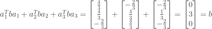
and the dot product of the second and third rows is zero:

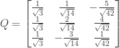
The resulting value for the matrix

The dot product of the first column with itself is

The dot product of the second column with itself is

The dot product of the third column with itself is

Thus all three columns have length 1.
We also have the dot product of the first and second columns as zero:

the dot product of the first and third columns as zero:

and the dot product of the second and third columns as zero:

Since all three rows are orthonormal (by construction) and all three columns are orthonormal, the matrix
Recall that we originally had two choices for the last entry of the first row. If we instead choose 

Verifying that this alternative value for
NOTE: This continues a series of posts containing worked out exercises from the (out of print) book Linear Algebra and Its Applications, Third Edition by Gilbert Strang.
If you find these posts useful I encourage you to also check out the more current Linear Algebra and Its Applications, Fourth Edition, Dr Strang’s introductory textbook Introduction to Linear Algebra, Fifth Edition
and the accompanying free online course, and Dr Strang’s other books
.
 and
and  , prove that
  ?
?


 the matrix


 and
and  , show that their product
  is also orthogonal. If
  and
and  , what does
  and
and  can be found in multiplying
 the matrix
  , and will contain elements including

 and
and  come from
  and
and  come from
 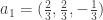 and
and 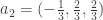 and the vector
  from the previous exercise, project
  onto a third orthonormal vector
  . What is the sum of the three projections? Why? Why is the matrix
  equal to the identity matrix
  ?
? is orthonormal, the projection of
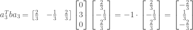
 ,
,  , and
, and  , and any vector
  in
in 
 , etc., are scalars) so that the 3 by 3 matrix
 of
of 


 to the data.
 .
. as follows:


 to create a system of the form
  . We have

 and from the first equation we have
  .
. with slope of 1 and
  -intercept of -2. For the values of
  of -2, -1, 1, and 2 the values of
  .
. , and the projection
  (in feet) at forces
  (in tons), and assuming that Hooke’s Law
  applies, use least squares to find the man’s length
  when no force is applied.
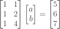

 and subtract it from the second equation to form the system
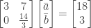
 and can substitute into the first equation to get
 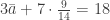 or
or
 or 4.5 feet.
 at
at  from the previous exercise, what would be the coefficient matrix
  , and the data vector
  ?
? and add a third column to the coefficient matrix
  for the various measurements. The vector


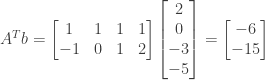
 and subtract it from the second equation to form the system
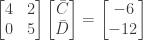
 and can substitute into the first equation to get
  or
or
 .
. show that the best least squares fit to the horizontal line
  is given by
 by 1 matrix with all entries equal to 1 and
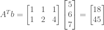
  . To find the least squares solution we form the system
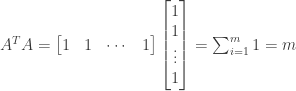

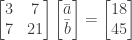
 so that

