Exercise 3.3.11. Suppose that  is a subspace with orthogonal complement
  , with
  a projection matrix onto and
  a projection matrix onto . What are
  and
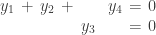
and  ? Also, show that
  is its own inverse.
Answer: Given any vector  we have
  where
where  is the projection of onto and
  is the projection of onto . Since and
  are orthogonal complements the sum of the projections and is equal to itself. So we have
  and since this is true for all we have
  .
.
This can be more formally proved as follows: Consider the matrix  . It is a projection matrix and it projects onto . Also, if is a projection matrix onto then it is unique. Since is a projection matrix onto and is a projection matrix onto we therefore have
  or . For the full proof see below.
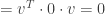
Since  we have
 .
.
(Applying to a vector first projects onto and then projects the resulting vector onto . But projecting any vector in onto will produce the zero vector, since and are orthogonal.)
Finally, we have
![(P-Q)(P-Q) = [(I-Q) - Q][(I-Q) - Q]](https://s0.wp.com/latex.php?latex=%28P-Q%29%28P-Q%29+%3D+%5B%28I-Q%29+-+Q%5D%5B%28I-Q%29+-+Q%5D&bg=ffffff&fg=333333&s=0&c=20201002)

Since  we have
  so that is its own inverse.
Here is the full proof that if a projection matrix onto and a projection matrix onto then :
We first show that is a projection matrix. The identity matrix  is symmetric, and since is a projection matrix it is also symmetric. The difference is therefore symmetric as well, so that we have
  .
.
We also have


Since and  we see that is a projection matrix.
Onto what subspace does project? For any vector we have  . Since is a projection matrix the vector is in the space onto which projects, and the vector
  is orthogonal to that space. But projects onto so
  must therefore be in
  .
.
We have thus shown that is a projection matrix that projects onto . We now show that any such projection matrix is unique.
Suppose that like the matrix  is also a projection matrix onto . Consider the vector
  for any vector . We have
![\|(P - P')v\|^2 = [(P-P')v]^T[(P-P')v]](https://s0.wp.com/latex.php?latex=%5C%7C%28P+-+P%27%29v%5C%7C%5E2+%3D+%5B%28P-P%27%29v%5D%5ET%5B%28P-P%27%29v%5D&bg=ffffff&fg=333333&s=0&c=20201002)

where we take advantage of the fact that  .
.
But since and are projection matrices they are symmetric, and therefore their difference  is also symmetric. We thus have

![= v^T[P^2 - PP' - P'P + (P')^2]v](https://s0.wp.com/latex.php?latex=%3D+v%5ET%5BP%5E2+-+PP%27+-+P%27P+%2B+%28P%27%29%5E2%5Dv&bg=ffffff&fg=333333&s=0&c=20201002)
But since and are projection matrices we have  and
and  . We thus have
![\|(P - P')v\|^2 = v^T[P - PP' - P'P + P']v](https://s0.wp.com/latex.php?latex=%5C%7C%28P+-+P%27%29v%5C%7C%5E2+%3D%C2%A0v%5ET%5BP+-+PP%27+-+P%27P+%2B+P%27%5Dv&bg=ffffff&fg=333333&s=0&c=20201002)
Since is a projection matrix onto we know that  for any vector
  in . (In other words, when applied to any vector in the projection matrix projects that vector onto itself.) The same is true for since it is also a projection matrix onto . We thus have
  for all in .
Given any vector (not necessarily in ) we then have  since is a vector in . Since is a projection matrix we have
  and thus
  , so that
  for all vectors . This implies that
  .
.
Similarly for any vector we have  since
since  is a vector in . Since is a projection matrix we have
  and thus
  , so that
  for all vectors . This implies that
  .
.
Since and we have

Since  we have
  , and since this is true for any vector we must have
  or
or  . A projection matrix onto a subspace is therefore unique.
Thus since is a projection matrix onto and is also a projection matrix onto we have or  .
.
NOTE: This continues a series of posts containing worked out exercises from the (out of print) book Linear Algebra and Its Applications, Third Edition by Gilbert Strang.
If you find these posts useful I encourage you to also check out the more current Linear Algebra and Its Applications, Fourth Edition , Dr Strang’s introductory textbook Introduction to Linear Algebra, Fifth Edition
 and the accompanying free online course, and Dr Strang’s other books
 .
.


 ,
,  , and
, and  ? What is the projection of

 of
of 
 as discussed above.
 .
. then what is the subspace onto which
  . We have
 we then have
 the matrix
  . So
. So  onto a subspace
  . What is the column space of
  . Since any vector in
  .
. . Consider the vector
  . We then have
  by the definition of
  for some
  .
. : The column space of
  and
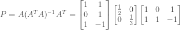
and  find the projection matrix


 of two orthogonal vectors
  where
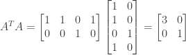
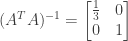
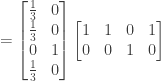
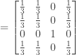
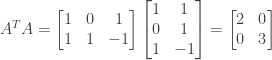
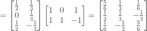
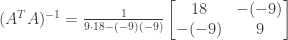
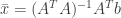
where 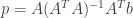 per equation (3) of 3L on page 156. We first compute
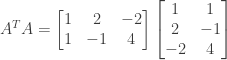


 we have
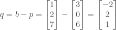

 , the column space of A, and the orthogonal subspace of
  , the left nullspace of
  . We confirm this:


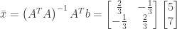
 , the least squares solution to
  that minimizes the error vector
  .
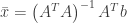
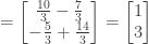
. . In this case we have
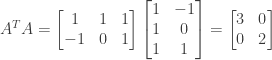


 with slope
  and intercept
  .
.

 , compute its partial derivatives with respect to
  and
and  to confirm that you obtain the same normal equations in both cases (i.e., using calculus vs. geometry). Then find the projection
  and explain why
  .
.


![= (u-1)^2 + (v-3)^2 + [(u+v)-4]^2](https://s0.wp.com/latex.php?latex=%3D+%28u-1%29%5E2+%2B+%28v-3%29%5E2+%2B+%5B%28u%2Bv%29-4%5D%5E2&bg=ffffff&fg=333333&s=0&c=20201002)
![= (u^2-2u+1) + (v^2-6v+9) +[ (u+v)^2 - 8(u+v) + 16]](https://s0.wp.com/latex.php?latex=%3D+%28u%5E2-2u%2B1%29+%2B+%28v%5E2-6v%2B9%29+%2B%5B+%28u%2Bv%29%5E2+-+8%28u%2Bv%29+%2B+16%5D&bg=ffffff&fg=333333&s=0&c=20201002)


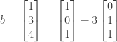
 and
and  represent the least squares solution.


 . We have
 by
by 

 is orthogonal to every column in