Linear Algebra and Its Applications, Exercise 1.7.3

Exercise 1.7.3. Given the differential equation

$- \frac{d^2u}{dx^2} = f(x), \quad \frac{du}{dx}(0) = \frac{du}{dx}(1) = 0$

what is the finite-difference matrix for $h = \frac{1}{6}$ (corresponding to a 5 by 5 matrix)? Note that you can replace the boundary condition $\frac{du}{dx}(0) = 0$ by $u_1 - u_0 = 0$ (and hence $u_1 = u_0$ ) and the boundary condition $\frac{du}{dx}(1) = 0$ by $u_6 - u_5 = 0$ (and hence $u_6 = u_5$ ).

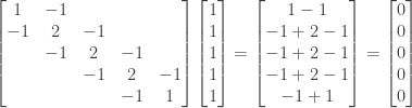
Show that the finite-difference matrix applied to the vector $(1, 1, 1, 1, 1)$ yields zero. Similarly, show that for any solution $u(x)$ to the original differential equation, $u(x) + 1$ is also a solution.

Answer: We can express $- \frac{d^2u}{dx^2} = f(x)$ in finite difference terms as

$- [u_{j-1} - 2u_j + u_j+1]/h^2 = f(jh)$

$\rightarrow -u_{j-1} + 2u_j - u_{j+1} = h^2 f(jh)$

We have $h = \frac{1}{6}$ and are thus considering meshpoints $x = jh, 0 \le j \le 6$ . The above equation can then be rewritten as

$-u_{j-1} + 2u_j - u_{j+1} = (\frac{1}{6})^2 f(jh) = \frac{1}{36} f(jh)$

where $u_j$ is the approximation of $u(x)$ at the point $x = jh$ .

We already know that $u_1 = u_0$ so that for $j = 1$ the above equation becomes

$-u_0 + 2u_1 - u_2 = \frac{1}{36} f(\frac{1}{6}) \rightarrow u_1 - u_2 = \frac{1}{36} f(\frac{1}{6})$

For $j = 2$ the above equation becomes

$-u_1 +2u_2 - u_3 = \frac{1}{36} f(\frac{2}{6}) = \frac{1}{36} f(\frac{1}{3})$

The equation has a similar form for $j = 3$ , $j = 4$ , and $j = 5$ . Since $u_6 = u_5$ for $j = 5$ the equation becomes

$-u_4 + 2u_5 - u_6 = \frac{1}{36} f(\frac{5}{6}) \rightarrow -u_4 + u_5 = \frac{1}{36} f(\frac{5}{6})$

The corresponding 5 by 5 finite-difference matrix is then

$\begin{bmatrix} 1&-1&&& \\ -1&2&-1&& \\ &-1&2&-1& \\ &&-1&2&-1 \\ &&&-1&1 \end{bmatrix} \begin{bmatrix} u_1 \\ u_2 \\ u_3 \\ u_4 \\ u_5 \end{bmatrix} = \frac{1}{36} \begin{bmatrix} f(\frac{1}{6}) \\ f(\frac{1}{3}) \\ f(\frac{1}{2}) \\ f(\frac{2}{3}) \\ f(\frac{5}{6}) \end{bmatrix}$

If we apply the finite-difference matrix to the constant vector $(1, 1, 1, 1, 1)$ we obtain the following:

$\begin{bmatrix} 1&-1&&& \\ -1&2&-1&& \\ &-1&2&-1& \\ &&-1&2&-1 \\ &&&-1&1 \end{bmatrix} \begin{bmatrix} 1 \\ 1 \\ 1 \\ 1 \\ 1 \end{bmatrix} = \begin{bmatrix} 1 - 1 \\ -1 + 2 - 1 \\ -1 + 2 - 1 \\ -1 + 2 - 1 \\ -1 + 1 \end{bmatrix} = \begin{bmatrix} 0\\ 0 \\ 0 \\ 0 \\ 0 \end{bmatrix}$

Finally, assume that $u(x)$ is a solution of $- \frac{d^2u}{dx^2} = f(x)$ and let $v(x) = u(x) + 1$ . Then we have

$-\frac{d^2v}{dx^2} = -\frac{d^2}{dx^2} [u(x) + 1] = -\frac{d^2}{dx^2}u(x) - \frac{d^2}{dx^2}(1)$

$= -\frac{d^2u}{dx^2} - 0 = -\frac{d^2u}{dx^2} = f(x)$

We also have

$\frac{dv}{dx}(0) = \frac{d}{dx}[u(0) + 1] = \frac{d}{dx}u(o) + \frac{d}{dx}(1) = \frac{du}{dx}(o) + 0 = \frac{du}{dx}(o) = 0$

and

$\frac{dv}{dx}(1) = \frac{d}{dx}[u(1) + 1] = \frac{d}{dx}u(1) + \frac{d}{dx}(1) = \frac{du}{dx}(1) + 0 = \frac{du}{dx}(1) = 0$

So $v(x) = u(x) + 1$ is also a solution if $u(x)$ is.

NOTE: This continues a series of posts containing worked out exercises from the (out of print) book Linear Algebra and Its Applications, Third Edition by Gilbert Strang.

If you find these posts useful I encourage you to also check out the more current Linear Algebra and Its Applications, Fourth Edition, Dr Strang’s introductory textbook Introduction to Linear Algebra, Fourth Edition and the accompanying free online course, and Dr Strang’s other books.

Linear Algebra and Its Applications, Exercise 1.7.3

Leave a Reply Cancel reply

Archives

Meta

Linear Algebra and Its Applications, Exercise 1.7.3

Share this:

Like this:

Related

Leave a Reply Cancel reply

Archives

Meta