
Exercise 1.7.5. What would the difference matrix in equation (6) look like if the boundary conditions were 


Answer: The finite difference equation would still be as given in equation (5):

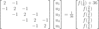
For 

![\rightarrow -u_2 + 2u_1 = h^2 f(jh) + 1 = h^2 [f(jh) + \frac{1}{h^2}]](https://s0.wp.com/latex.php?latex=%5Crightarrow+-u_2+%2B+2u_1+%3D+h%5E2+f%28jh%29+%2B+1+%3D+h%5E2+%5Bf%28jh%29+%2B+%5Cfrac%7B1%7D%7Bh%5E2%7D%5D&bg=ffffff&fg=333333&s=0&c=20201002)
Since 
NOTE: This continues a series of posts containing worked out exercises from the (out of print) book Linear Algebra and Its Applications, Third Edition by Gilbert Strang.
If you find these posts useful I encourage you to also check out the more current Linear Algebra and Its Applications, Fourth Edition, Dr Strang’s introductory textbook Introduction to Linear Algebra, Fourth Edition
and the accompanying free online course, and Dr Strang’s other books
.

