Linear Algebra and Its Applications, Exercise 2.2.12

Exercise 2.2.12. What is a 2 by 3 system of equations $Ax = b$ that has the following general solution?

$x = \begin{bmatrix} 1 \\ 1 \\ 0 \end{bmatrix} + w \begin{bmatrix} 1 \\ 2 \\ 1 \end{bmatrix}$

Answer: The general solution above is the sum of a particular solution and a homogeneous solution, where

$x_{particular} = \begin{bmatrix} 1 \\ 1 \\ 0 \end{bmatrix}$

and

$x_{homogeneous} = w \begin{bmatrix} 1 \\ 2 \\ 1 \end{bmatrix}$

Since $w$ is the only variable referenced in the homogeneous solution it must be the only free variable, with $u$ and $v$ being basic. Since $u$ is basic we must have a pivot in column 1, and since $v$ is basic we must have a second pivot in column 2. After performing elimination on $A$ the resulting echelon matrix $U$ must therefore have the form

$U = \begin{bmatrix} *&*&* \\ 0&*&* \end{bmatrix}$

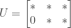
To simplify solving the problem we can assume that $A$ also has this form; in other words, we assume that $A$ is already in echelon form and thus we don’t need to carry out elimination. The matrix $A$ then has the form

$A = \begin{bmatrix} a_{11}&a_{12}&a_{13} \\ 0&a_{22}&a_{23} \end{bmatrix}$

where $a_{11}$ and $a_{22}$ are nonzero (because they are pivots).

We then have

$Ax_{homogeneous} = \begin{bmatrix} a_{11}&a_{12}&a_{13} \\ 0&a_{22}&a_{23} \end{bmatrix} w \begin{bmatrix} 1 \\ 2 \\ 1 \end{bmatrix} = 0$

If we assume that $w$ is 1 and express the right-hand side in matrix form this then becomes

$\begin{bmatrix} a_{11}&a_{12}&a_{13} \\ 0&a_{22}&a_{23} \end{bmatrix} \begin{bmatrix} 1 \\ 2 \\ 1 \end{bmatrix} = \begin{bmatrix} 0 \\ 0 \end{bmatrix}$

or (expressed as a system of equations)

$\setlength\arraycolsep{0.2em}\begin{array}{rcrcrcl}a_{11}&+&2a_{12}&+&a_{13}&=&0 \\ &&2a_{22}&+&a_{23}&=&0 \end{array}$

The pivot $a_{11}$ must be nonzero, and we arbitrarily assume that $a_{11} = 1$ . We can then satisfy the first equation by assigning $a_{12} = 0$ and $a_{13} = -1$ . The pivot $a_{22}$ must also be nonzero, and we arbitrarily assume that $a_{22} = 1$ as well. We can then satisfy the second equation by assigning $a_{23} = -2$ . Our proposed value of $A$ is then

$A = \begin{bmatrix} 1&0&-1 \\ 0&1&-2 \end{bmatrix}$

so that we have

$Ax_{homogeneous} = \begin{bmatrix} 1&0&-1 \\ 0&1&-2 \end{bmatrix} \begin{bmatrix} 1 \\ 2 \\ 1 \end{bmatrix} = \begin{bmatrix} 0 \\ 0 \end{bmatrix}$

as required.

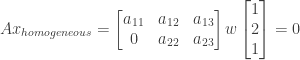
We next turn to the general system $Ax = b$ . We now have a value for $A$ , and we were given the value of the particular solution. We can multiply the two to calculate the value of $b$ :

$b = Ax_{particular} = \begin{bmatrix} 1&0&-1 \\ 0&1&-2 \end{bmatrix} \begin{bmatrix} 1 \\ 1 \\ 0 \end{bmatrix} = \begin{bmatrix} 1 \\ 1 \end{bmatrix}$

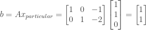
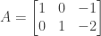
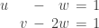
This gives us the following as an example 2 by 3 system that has the general solution specified above:

$\begin{bmatrix} 1&0&-1 \\ 0&1&-2 \end{bmatrix} \begin{bmatrix} u \\ v \\ w \end{bmatrix} = \begin{bmatrix} 1 \\ 1 \end{bmatrix}$

$\setlength\arraycolsep{0.2em}\begin{array}{rcrcrcl}u&&&-&w&=&1 \\ &&v&-&2w&=&1 \end{array}$

Finally, note that the solution provided for exercise 2.2.12 at the end of the book is incorrect. The right-hand side must be a 2 by 1 matrix and not a 3 by 1 matrix, so the final value of 0 in the right-hand side should not be present.

NOTE: This continues a series of posts containing worked out exercises from the (out of print) book Linear Algebra and Its Applications, Third Edition by Gilbert Strang.

If you find these posts useful I encourage you to also check out the more current Linear Algebra and Its Applications, Fourth Edition, Dr Strang’s introductory textbook Introduction to Linear Algebra, Fourth Edition and the accompanying free online course, and Dr Strang’s other books.

This entry was posted in linear algebra. Bookmark the permalink.

2 Responses to Linear Algebra and Its Applications, Exercise 2.2.12

Daniel says:

May 24, 2012 at 6:46 am

I think that your final note is incorrect, due to the fact that if you find the general solution for the system Ax=b that you found, you’ll have to write the solution like Strang does it in (3) page (76). There are three entries on the solution because “x” vector lenght. The general solution (in Matlab notation) is x = [u; v; w] = [1+w; 1+2w; w]= [1; 1; 0] + w*[1; 2; 1]. The general solution he proposed at the begining of the exercise

- hecker says:
  
  May 26, 2012 at 1:23 pm
  
  My apologies for the delay in responding. Are you referring to my final sentence about the solution to exercise 2.2.12 given on page 476 in the back of the book? If so, I think I may have confused you. I am *not* saying that Strang wrote the general solution incorrectly in the statement of the exercise on page 79, or that Strang found an incorrect solution to the exercise.
  
  Rather my point is as follows: In the statement of the solution on page 476 Strang shows as a solution the same 2 by 3 matrix that I derived above, and Strang shows that 2 by 3 matrix multiplying the vector (u, v, w) just as I do above, representing a system of two equations in three unknowns. However on the right-hand side Strang shows that 2 by 3 matrix multiplying the vector (u, v, w) to produce the vector (1, 1, 0). This cannot be: since the matrix has only two rows, that multiplication would produce a vector with only two elements, not three (as in the book). Those two elements represent the right-hand sides of the corresponding system of two equations.
  
  So the left-hand side in the solution of 2.2.12 on page 476 is correct, but the right-hand side of the solution of 2.2.12 on page 476, namely the vector (1, 1, 0), is not. Instead the right-hand side should be the vector (1, 1) as I derived above.