Exercise 2.2.13. What is a 3 by 3 system of equations  that has the following general solution (the same as in exercise 2.2.12)

and that has no solution if  ?
?
Answer: As in exercise 2.2.12, the general solution above is the sum of a particular solution and a homogeneous solution, where

and

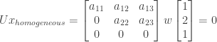
Also as in exercise 2.2.12, since  is the only variable referenced in the homogeneous solution it must be the only free variable, with
  and
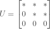
and  being basic. Since is basic we must have a pivot in column 1, and since is basic we must have a second pivot in column 2. After performing elimination on
  the resulting echelon matrix
  must therefore have the form
Unlike in exercise 2.2.12 we cannot simply assume that  because we need to account for the particular condition
  that is required for the system to have a solution. This condition arises from the particular sequence of elimination steps that takes the system and produces the equivalent system
  with
with  resulting from the elimination operations applied to
  . In particular, we assume that the system will look as follows:

The third row produces the equation  or . This corresponds to the assumption that there is no solution if .
We can’t assume that but we can assume that the first two rows of are the same as the first two rows of . That removes the need to do elimination for the second row of and corresponds to our assumption that the second element of is the same as the second element of (namely  ). We then have to do elimination operations only for the third row, and those operations will produce the third element of as listed above.
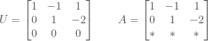
As stated above the general solution to for this exercise is the same as the general solution in exercise 2.2.12, so the homogeneous solution is the same as well. Since we are assuming that the first two rows of are the same as the first two rows of we have
Note that the first two rows produce the same equations as in exercise 2.2.12. The third row is simply equivalent to the equation  and so adds no new information. We can therefore follow the same process as in exercise 2.2.12 to find values for the first two rows of and :
so that we have

We now turn to determining the last row of :

In order to produce  as the last element of on the right-hand side (i.e., of ) we must subtract the first row from the third row on the left-hand side to produce a zero as the first element of the third row, and then subsequently subtract the second row from the third row to produce a zero as the second element of the third row. That first operation means we must have
  or
or  . The second operation means we must have
 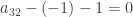 or
or  as well as
  or
or  . The proposed value for is then
We next turn to the general system . We now have a value for , and we were given the value of the particular solution. We can multiply the two to calculate the value of :

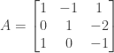
This gives us the following as an example 3 by 3 system that has the general solution specified above:
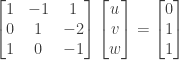
or

Note that we have  . If this were not the case then the system would have no solution.
NOTE: This continues a series of posts containing worked out exercises from the (out of print) book Linear Algebra and Its Applications, Third Edition by Gilbert Strang.
If you find these posts useful I encourage you to also check out the more current Linear Algebra and Its Applications, Fourth Edition , Dr Strang’s introductory textbook Introduction to Linear Algebra, Fourth Edition
 and the accompanying free online course, and Dr Strang’s other books
 .
.


I quess that’s not the only 3 by 3 system that has the above general solution,right?
That’s a good question. I did make some assumptions as to the form of A relative to U, and it’s possible that if you change those assumptions then it’s possible to find different values for A and b. However I have not tried to do this myself.