Exercise 2.4.18. Given the vectors

and the subspace that they span, find two matrices and such that .

Answer: The easiest way to create a matrix whose row space is is to use the vectors above as the rows of the matrix:

However we can simplify things by doing Gaussian elimination on this matrix to obtain another matrix with the same row space , first subtracting the first row from the second and third rows, and then subtracting four times the second row from the third:

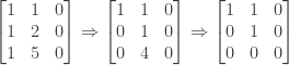
We can then further simplify by subtracting the second row from the first; again, this does not change the row space:

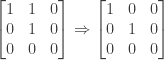
Our final matrix is thus

with . Note that is the x-y plane in and the coordinate vectors and are a basis for .

We now want to find a second matrix whose nullspace is . If then for any vector in we must have . In particular, we must have for the coordinate vectors and that form a basis for . The simplest way to define B is then as the 1 by 3 matrix

for which

and

For any solution to we must then have

From the above we see that and that and can take on any value. The nullspace therefore contains all vectors of the form

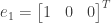
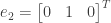
But this is equivalent to all linear combinations of the coordinate vectors and that form a basis for . We thus have .

NOTE: This continues a series of posts containing worked out exercises from the (out of print) book Linear Algebra and Its Applications, Third Edition by Gilbert Strang.

If you find these posts useful I encourage you to also check out the more current Linear Algebra and Its Applications, Fourth Edition, Dr Strang’s introductory textbook Introduction to Linear Algebra, Fourth Edition and the accompanying free online course, and Dr Strang’s other books.

 Buy me a snack to sponsor more posts like this!