Linear Algebra and Its Applications, Exercise 2.5.6

Exercise 2.5.6. Determine the incidence matrix $A$ for the graph on page 113 with six edges and four nodes, as follows: Edge 1 from node 1 to node 2, edge 2 from node 1 to node 3, edge 3 from node 2 to node 3, edge 4 from node 2 to node 4, edge 5 from node 1 to node 4, and edge 6 from node 3 to node 4.

Find three independent vectors $y$ that satisfy $A^Ty = 0$ . How do these vectors relate to the loops in the graph?

Answer: Since there are six edges in the graph the incidence matrix $A$ has six rows, and since there are four nodes $A$ has four columns; $A$ is therefore a 6 by 4 matrix.

The first row of $A$ corresponds to edge 1. Since edge 1 goes from node 1 to node 2 the entry in the (1, 1) position is -1 (representing “flow” out of node 1) and the entry in the (1, 2) position is 1 (representing flow into node 2). Since edge 2 goes from node 1 to node 3 the entry in the (2, 1) position is -1 (representing flow out of node 1) and the entry in the (2, 3) position is 1 (representing flow into node 3). The values of the entries for the other rows (edges) can be similarly determined, and the final incidence matrix is

$A = \begin{bmatrix} -1&1&0&0 \\ -1&0&1&0 \\ 0&-1&1&0 \\ 0&-1&0&1 \\ -1&0&0&1 \\ 0&0&-1&1 \end{bmatrix}$

We now try to find a solution to $A^Ty = 0$ or

$\begin{bmatrix} -1&-1&0&0&-1&0 \\ 1&0&-1&-1&0&0 \\ 0&1&1&0&0&-1 \\ 0&0&0&1&1&1 \end{bmatrix} \begin{bmatrix} y_1 \\ y_2 \\ y_3 \\ y_4 \\ y_5 \\ y_6 \end{bmatrix} = \begin{bmatrix} 0 \\ 0 \\ 0 \\ 0 \end{bmatrix}$

by doing Gaussian elimination on $A^T$ .

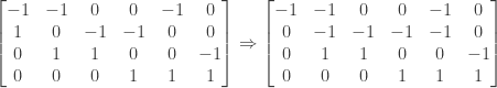
We first subtract -1 times the first row from the second row:

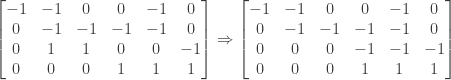
$\begin{bmatrix} -1&-1&0&0&-1&0 \\ 1&0&-1&-1&0&0 \\ 0&1&1&0&0&-1 \\ 0&0&0&1&1&1 \end{bmatrix} \Rightarrow \begin{bmatrix} -1&-1&0&0&-1&0 \\ 0&-1&-1&-1&-1&0 \\ 0&1&1&0&0&-1 \\ 0&0&0&1&1&1 \end{bmatrix}$

We then subtract -1 times the second row from the third row:

$\begin{bmatrix} -1&-1&0&0&-1&0 \\ 0&-1&-1&-1&-1&0 \\ 0&1&1&0&0&-1 \\ 0&0&0&1&1&1 \end{bmatrix} \Rightarrow \begin{bmatrix} -1&-1&0&0&-1&0 \\ 0&-1&-1&-1&-1&0 \\ 0&0&0&-1&-1&-1 \\ 0&0&0&1&1&1 \end{bmatrix}$

Finally, we subtract -1 times the third row from the fourth row:

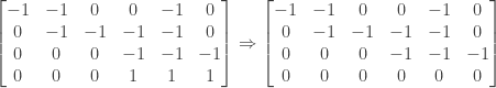
$\begin{bmatrix} -1&-1&0&0&-1&0 \\ 0&-1&-1&-1&-1&0 \\ 0&0&0&-1&-1&-1 \\ 0&0&0&1&1&1 \end{bmatrix} \Rightarrow \begin{bmatrix} -1&-1&0&0&-1&0 \\ 0&-1&-1&-1&-1&0 \\ 0&0&0&-1&-1&-1 \\ 0&0&0&0&0&0 \end{bmatrix}$

The resulting echelon matrix has pivots in columns one, two, and four, so $y_1$ , $y_2$ , and $y_4$ are basic variables and $y_3$ , $y_5$ , and $y_6$ are free variables.

We first set $y_3 = 1$ and $y_5 = y_6 = 0$ . From the third row of the echelon matrix we have

$-y_4 - y_5 - y_6 = 0 \rightarrow y_4 - 0 - 0 = 0$

$\rightarrow y_4 = 0$

From the second row of the echelon matrix we have

$-y_2 - y_3 - y_4 - y_5 = 0 \rightarrow -y_2 - 1 - 0 - 0 = 0$

$\rightarrow y_2 = -1$

and from the first row we then have

$-y_1 - y_2 - y_5 = 0 \rightarrow -y_1 - (-1) = 0$

$\rightarrow y_1 = 1$

So one solution to $A^Ty = 0$ is $\begin{bmatrix} 1&-1&1&0&0&0 \end{bmatrix}^T$ .

We next set $y_5 = 1$ and $y_3 = y_6 = 0$ . From the third row of the echelon matrix we have

$-y_4 - y_5 - y_6 = 0 \rightarrow -y_4 - 1 - 0 = 0$

$\rightarrow y_4 = -1$

From the second row of the echelon matrix we have

$-y_2 - y_3 - y_4 - y_5 = 0 \rightarrow -y_2 - 0 - (-1) - 1 = 0$

$\rightarrow y_2 = 0$

and from the first row we then have

$-y_1 - y_2 - y_5 = 0 \rightarrow -y_1 - 0 - 1 = 0$

$\rightarrow y_1 = -1$

So a second solution to $A^Ty = 0$ is $\begin{bmatrix} -1&0&0&-1&1&0 \end{bmatrix}^T$ .

Finally we set $y_6 = 1$ and $y_3 = y_5 = 0$ . From the third row of the echelon matrix we have

$-y_4 - y_5 - y_6 = 0 \rightarrow -y_4 - 0 - 1 = 0$

$\rightarrow y_4 = -1$

From the second row of the echelon matrix we have

$-y_2 - y_3 - y_4 - y_5 = 0 \rightarrow -y_2 - 0 - (-1) - 0 = 0$

$\rightarrow y_2 = 1$

and from the first row we then have

$-y_1 - y_2 - y_5 = 0 \rightarrow -y_1 - 1 - 0 = 0$

$\rightarrow y_1 = -1$

So a third solution to 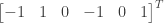$A^Ty = 0$ is $\begin{bmatrix} -1&1&0&-1&0&1 \end{bmatrix}^T$ .

The following set of three vectors $u$ , $v$ , and $w$ are thus solutions to $A^Ty = 0$ . The vectors are independent (as you can verify by inspecting them):

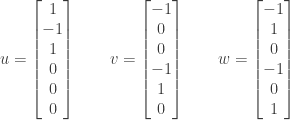
$u = \begin{bmatrix} 1 \\ -1 \\ 1 \\ 0 \\ 0 \\ 0 \end{bmatrix} \qquad v = \begin{bmatrix} -1 \\ 0 \\ 0 \\ -1 \\ 1 \\ 0 \end{bmatrix} \qquad w = \begin{bmatrix} -1 \\ 1 \\ 0 \\ -1 \\ 0 \\ 1 \end{bmatrix}$

Since $A^Ty = y^TA$ the vectors are in the left nullspace of $A$ . (In fact they form a basis for the left nullspace.)

The vectors also correspond to independent loops in the graph used to create the incidence matrix $A$ :

The first vector $u$ is a loop around the outside of the graph, and includes edge 1, edge 2, and edge 3. Note that edge 2 runs in a different direction than the other two, and hence its corresponding entry is reversed in sign from the other two.

The second vector $v$ is a loop around an interior triangle of the graph (in the upper left), and includes edge 1, edge 4, and edge 5, with edge 5 running in a different direction than the other two.

The third vector $w$ includes edges 1, 2, 4, and 6, with edges 2 and 6 running in different directions than the other two.

Note that if we add $u$ and $w$

$u + w = \begin{bmatrix} 1 \\ -1 \\ 1 \\ 0 \\ 0 \\ 0 \end{bmatrix} + \begin{bmatrix} -1 \\ 1 \\ 0 \\ -1 \\ 0 \\ 1 \end{bmatrix} = \begin{bmatrix} 0 \\ 0 \\ 1 \\ -1 \\ 0 \\ 1 \end{bmatrix}$

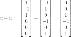
we get a vector representing a loop around the bottom interior triangle of the graph, comprising edges 3, 4, and 6.

Similarly, if we subtract $v$ from $w$

$w - v = \begin{bmatrix} -1 \\ 1 \\ 0 \\ -1 \\ 0 \\ 1 \end{bmatrix} - \begin{bmatrix} -1 \\ 0 \\ 0 \\ -1 \\ 1 \\ 0 \end{bmatrix} = \begin{bmatrix} 0 \\ 1 \\ 0 \\ 0 \\ -1 \\ 1 \end{bmatrix}$

we get a vector representing the loop around the upper right interior triangle, comprising edges 2, 5, and 6.

These two vectors together with $v$ thus represent independent loops associated with the three interior triangles of the graph.

NOTE: This continues a series of posts containing worked out exercises from the (out of print) book Linear Algebra and Its Applications, Third Edition by Gilbert Strang.

If you find these posts useful I encourage you to also check out the more current Linear Algebra and Its Applications, Fourth Edition, Dr Strang’s introductory textbook Introduction to Linear Algebra, Fourth Edition and the accompanying free online course, and Dr Strang’s other books.

Buy me a snack to sponsor more posts like this!

Linear Algebra and Its Applications, Exercise 2.5.6

Leave a Reply Cancel reply

Archives

Meta

Linear Algebra and Its Applications, Exercise 2.5.6

Share this:

Like this:

Related

Leave a Reply Cancel reply

Archives

Meta