Exercise 2.5.7. Suppose that the incidence matrix from exercise 2.5.6 (for the graph on page 113 with six edges and four nodes) represents six games among four teams, and that the score differences for the six games are through . When you can assign potentials to the teams so that the potentials agree with the values of through ?

(This corresponds to finding conditions on through that make the system solvable. These can be found via elimination or by using Kirchoff’s Laws.)

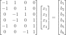
Answer: We first attempt to solve using Gaussian elimination, starting with the original system of equations:

We start by subtracting 1 times the first row from the second and fifth rows:

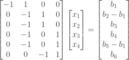
We then subtract 1 times the second row from the third, fourth, and fifth rows:

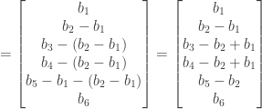
Finally we subtract 1 times the fourth row from the fifth and sixth rows:

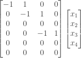
From the third row we see that we must have . From the fifth row we must have . Finally, from the sixth row we must have . Rearranging the terms to put them in order and multiplying the second and third equations by -1 gives us the following three conditions:

Now we try to find conditions on through by using Kirchoff’s Law of Voltages. Recall from exercise 2.5.6 that we found three independent loops in the graph, the first running around the outer edges, the second around the interior triangle in the upper left of the graph, and the third including edges 1, 2, 4, and 6.

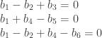
The outer loop of the graph contains edges 1, 2, and 3, with edge 2 running in the opposite direction from the other two. Since , , and are the potential differences along each edge, and the sum of the potential differences around the loop must be zero, we must have . This gives us the first condition listed above.

The loop around the interior triangle in the upper left contains edges 1, 4, and 5, with edge 5 running in the opposite direction from the other two. Since , , and are the potential differences along each edge, and the sum of the potential differences around the loop must be zero, we must have . This gives us the second condition listed above.

The final loop contains edges 1, 2, 4, and 6, with edges 2 and 6 running in the opposite direction from the other two. Since , , , and are the potential differences along each edge, and the sum of the potential differences around the loop must be zero, we must have . This gives us the third and final condition listed above.

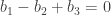
Note that by choosing a different set of independent loops we produce a different but equivalent set of conditions. For example, if we choose as the independent loops the three interior triangles of the graph (in the upper left, upper right, and bottom of the graph respectively) then the corresponding conditions are as follows:

The first condition is the same as the second condition in the original set.

Subtracting the second condition from the first produces the third condition in the original set:

Finally, subtracting the second condition from the first and then adding the third produces the first condition in the original set:

NOTE: This continues a series of posts containing worked out exercises from the (out of print) book Linear Algebra and Its Applications, Third Edition by Gilbert Strang.

If you find these posts useful I encourage you to also check out the more current Linear Algebra and Its Applications, Fourth Edition, Dr Strang’s introductory textbook Introduction to Linear Algebra, Fourth Edition and the accompanying free online course, and Dr Strang’s other books.

 Buy me a snack to sponsor more posts like this!