Review exercise 2.26. State whether the following statements are true or false:
a) For every subspace  of
of  there exists a matrix
  for which the nullspace of is .
b) For any matrix , if both and its transpose  have the same nullspace then is a square matrix.
c) The transformation from  to that transforms
  into
into  (for some scalars
  and
and  ) is a linear transformation.
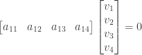
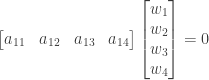
Answer: a) For the statement to be true, for any subspace of we must be able to find a matrix such that  . (In other words, for any vector in we have
  and for any such that the vector is an element of .)
What would such a matrix look like? First, since is a subspace of any vector in has four entries:  . If we have then the matrix must have four columns; otherwise would not be able to multiply from the left side.
Second, note that the nullspace of and the column space of are related: If the column space has dimension  then the nullspace of has dimension
  where
where  is the number of columns of . Since has four columns (from the previous paragraph) the dimension of
  is
is  .
.
Put another way, if  is the dimension of and is the nullspace of then we must have
  or
or  . So if the dimension of is
  then we have
  , if the dimension of is
  then we have
  , and so on.
Finally, if the matrix has rank then has both linearly independent columns and linearly independent rows. As noted above, the number of columns of (linearly independent or otherwise) is fixed by the requirement that the nullspace of should be a subspace of . So must always have four columns, and must have at least rows.
We now have five possible cases to consider, and can approach them as follows:
- has dimension 0 or 4. In both these cases there is only one possible subspace and we can easily find a matrix meeting the specified criteria.
- has dimension 1, 2, or 3. In each of these cases there are many possible subspaces (an infinite number, in fact). For a given we do the following:
- Start with a basis for . (Any basis will do.)
- Consider the effect on the basis vectors if they were to be in the nullspace of some matrix meeting the criteria above.
- Take the corresponding system of linear equations, re-express it as a system involving the entries of as unknowns and the entries of the basis vectors as coefficients, and show that we can solve the system to find the unknowns.
- Show that all other vectors in are also in the nullspace of .
- Show that any vector in the nullspace of must also be in .
We now proceed to the individual cases:
has dimension  . We then have
  . (If has dimension 4 then its basis has four linearly independent vectors. If
  then there must be some vector
  in but not in , and that vector must be linearly independent of the vectors in the basis of . But it is impossible to have five linearly independent vectors in a 4-dimensional vector space, so we conclude that .)
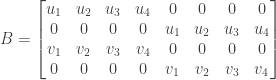
We then must have for any vector in . This is true when is equal to the zero matrix. As noted above must have exactly four columns and at least  rows. So one possible value for is

(The matrix could have additional rows as well, as long as they are all zeros.)
We have thus found a matrix such that any vector in is also in . Going the other way, any vector in must have four entries (in order for to be able to multiply it) so that any such vector is also in  .
.
So if is a 4-dimensional subspace (namely ) then a matrix exists such that is the nullspace of .
has dimension . The only 0-dimensional subspace of is that consisting only of the zero vector  . (If contained only a single nonzero vector then it would not be closed under multiplication, since multiplying that vector times the scalar 0 would produce a vector not in . If were not closed under multiplication then it would not be a subspace.)
In this case the matrix would have to have rank  . If
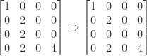
. If  then all four columns of would have to be linearly independent and would have to have at least four linearly independent rows. Suppose we choose the four elementary vectors
  through
  as the columns, so that

If we then have

so that the only solution is . We have thus again found a matrix for which .
(Note that any other matrix of rank would have worked as well: The product  is a linear combination of the columns of , with the coefficients being
  through
  . If the columns of are linearly independent then that linear combination can be zero only if all the coefficients through are zero.)
Having disposed of the easy cases, we now proceed to the harder ones.
has dimension  . In this case we are looking for a matrix with rank
  such that . The matrix thus must have only one linearly independent column and (more important for our purposes) only one linearly independent row. We need only find a matrix that is 1 by 4. (If desired we can construct suitable matrices that are 2 by 4, 3 by 4, etc., by adding additional rows that are multiples of the first row.)
Since the dimension of is 3, any three linearly independent vectors in form a basis for ; we pick an arbitrary set of such vectors  , , and
  . For to be equal to we must have
  ,
,  , and
, and  . We are looking for a matrix that is 1 by 4, so these equations correspond to the following:

These can in turn be rewritten as the following system of equations:

This is a system of three equations in four unknowns, equivalent to the matrix equation  where
where
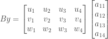
Since the vectors , , and are linearly independent (because they form a basis for the 3-dimensional subspace ) and the vectors in question form the rows of the matrix  , the rank of is . We also have
  , the number of rows of . Since this is true, per 20Q on page 96 there exists at least one solution
  to the above system . But is simply the first and only row in the matrix we were looking for, so this in turn means that we have found a matrix for which , , and are in the nullspace of .
If is a vector in then can be expressed as a linear combination of the basis vectors , , and for some set of coefficients  ,
,  , and
, and  . We then have


So any vector in is also an element in the nullspace of .
Suppose that is a vector in the nullspace of and is not in . Since is not in it cannot be expressed as a linear combination solely of the basis vectors , , and ; rather we must have

where  is some vector that is linearly independent of , , and .
If is in the nullspace of then we have  so
so


If  then either
  or
or  . If then we have

so that is actually an element of , contrary to our supposition. If then is an element of the nullspace of . But has dimension 3 and already contains the three linearly independent vectors , , and . The fourth vector cannot be both an element of and also linearly independent of , , and .
Our assumption that is in the nullspace of but is not in has thus led to a contradiction. We conclude that any element of is also in . We previously showed that any element of is also in , so we conclude that  .
.
For any 3-dimensional subspace of we can therefore find a matrix such that is the nullspace of .
has dimension  . In this case we are looking for a matrix with rank
  such that . The matrix thus must have only two linearly independent columns and only two linearly independent rows. We thus look for a matrix that is 2 by 4.
Since the dimension of is 2, any two linearly independent vectors in form a basis for ; we pick an arbitrary set of such vectors and . For to be equal to we must have and . We are looking for a matrix that is 2 by 4, so these equations correspond to the following:
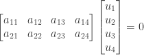

These can in turn be rewritten as the following system of four equations in eight unknowns:
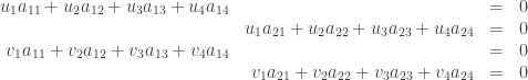
or where
Since the four rows are linearly independent (this follows from the linear independence of and ) we have so that the system is guaranteed to have a solution . The entries in are just the entries of so we have found a matrix for which the basis vectors and are members of the nullspace.
Since the basis vectors of are in all other elements of are in also. By the same argument as in the 3-dimensional case, any vector in must be in also; otherwise a contradiction occurs. Thus we conclude that .
For any 2-dimensional subspace of we can therefore find a matrix such that is the nullspace of .
has dimension . In this case we are looking for a matrix with rank  such that . The matrix thus must have only three linearly independent columns and only three linearly independent rows. We thus look for a matrix that is 3 by 4.
Since the dimension of is 1, any nonzero vector in forms a basis for . For to be equal to we must have . We are looking for a matrix that is 3 by 4, so this equation corresponds to the following:

This can be rewritten as a system of three equations with twelve unknowns ( ), a system which is guaranteed to have at least one solution due to the linear independence of the three rows of . The solution then forms the entries of , so that we have . Since is a basis for any other vector in is also in the nullspace of .
By the same argument as in the 3-dimensional case, any vector in must be in also; otherwise a contradiction occurs. Thus we conclude that .
For any 1-dimensional subspace of we can therefore find a matrix such that is the nullspace of .
Any subspace of must have dimension from 0 through 4. We have thus shown that for any subspace of we can find a matrix such that . The statement is true.
b) Suppose that for some by matrix both and its transpose have the same nullspace.
The rank of is also the rank of . The rank of is then , and the rank of  is
is  . Since
  we then have
  so that
  .
.
The number of rows of is the same as the number of columns of so that (and thus ) is a square matrix. The statement is true.
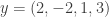
c) If  represents the transformation in question, with
  , we have


These two quantities are not the same unless  , so for
  the transformation is not linear. The statement is false.
NOTE: This continues a series of posts containing worked out exercises from the (out of print) book Linear Algebra and Its Applications, Third Edition by Gilbert Strang.
If you find these posts useful I encourage you to also check out the more current Linear Algebra and Its Applications, Fourth Edition , Dr Strang’s introductory textbook Introduction to Linear Algebra, Fourth Edition
 and the accompanying free online course, and Dr Strang’s other books
 .
.
 Buy me a snack to sponsor more posts like this!


 factorization:
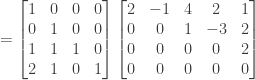
 has three pivots (in columns 1, 3, and 5) and thus has rank
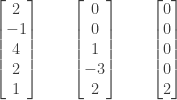


 .
. . From the echelon matrix
  and
and  are basic variables and that
  and
and  and
and  . From row 3 of
  . From row 2 we have
  or
or  . From row 1 we have
 . So one solution is
  .
. and
and  . From row 3 of
  or
or  . From row 1 we have
 . So a second solution is
  .
.
 such that for any vector
  .
.

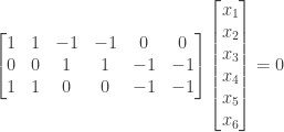


 are free variables.
 . From the second row of the echelon matrix we have
  or
or  or
or  . One solution to the system is thus
  .
. . From the second row of the echelon matrix we have
  or
or  . From the first row we have
  or
or  . A second solution to the system is thus
  .
. and
and  . From the second row of the echelon matrix we have
  or
or  . From the first row we have
  or
or  . A third solution to the system is thus
  .
. and
and  . From the second row of the echelon matrix we have
  or
or  or
or  .
.

 , the dimension of the nullspace is
  , and there cannot be more than four linearly independent vectors in the nullspace.)
 whose column space is the subspace simply by setting the columns of
 . Under what conditions would
  ?
? to exist
  and
and  .
.
 is 1 by
  is a 1 by 1 matrix, or in other words a scalar value

 . Another way is if
  . Note that this would be trivially true if
  to be zero even if
  and
and  so that
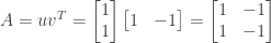


 so that
  (in other words,
  . Then we have
 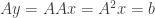 . Since there exists a
  we see that
 and
and  as a basis. Describe the effect of each transformation.
 is applied to the vector
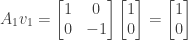

 is applied to the vector

 we obtain
 is applied to the vector
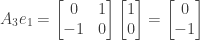

 has a solution for any
  . (In other words, the
  . The left nullspace thus contains only the zero vector.
 or
or  . Since the rank of
 .
.
 or
or  or
or  , and from the first equation we have
  or
or  . The vector
 and a basis for the nullspace of
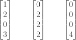
 .
. or (alternately)
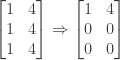
  . To do this we do Gaussian elimination on the matrix


 is a free variable and the rest are basic.
 , from the fourth equation we have
  or
or  , from the second equation we have
  or
or  , and from the first equation we have

 and the first column
 . In the homogeneous system
  or
or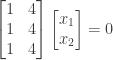
 or
or  . The vector

 .
. or (alternately)
  . To do this we do Gaussian elimination on the matrix

 and
and  and
and  , from the first equation we have
  or
or  . Setting
  or
or 
 and form a basis for the left nullspace of
