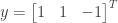
Exercise 2.5.1. Describe the incidence matrix 
The graph has three nodes and three edges, with edge 1 going from node 2 to node 1, edge 2 going from node 3 to node 2, and edge 3 going from node 3 to node 1.
Find a solution to 


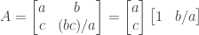
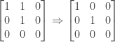
Answer: Since the graph has three edges the incidence matrix

The first row represents edge 1 from node 2 to node 1 (i.e., leaving node 2 and entering node 1). The second row represents edge 2 from node 3 to node 2. The third row represents edge 3 from node 3 to node 1.
The sum of the first and second rows equals the third row, so the rank 


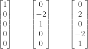
Since the entries in each row sum to zero, the vector 


Since 


UPDATE: Added a paragraph to clarify what the rows of
NOTE: This continues a series of posts containing worked out exercises from the (out of print) book Linear Algebra and Its Applications, Third Edition by Gilbert Strang.
If you find these posts useful I encourage you to also check out the more current Linear Algebra and Its Applications, Fourth Edition, Dr Strang’s introductory textbook Introduction to Linear Algebra, Fourth Edition
and the accompanying free online course, and Dr Strang’s other books
.
 the associated subspaces (column space, row space, null space, and left nullspace) are the same. Does this imply that
  ?
?
 . We also have the row spaces
  . Since the matrices are nonsingular the nullspaces
  contain only the zero vector and are thus equal. For the same reason the left nullspaces
  also contain only the zero vector and are also equal.
 for some scalar


 and the row space is all of
  .
. is to use the vectors in question as the only columns in the matrix:
 so that vector is in the row space
  . Similarly adding the first row of
  so that vector is also in the row space
  (since each vector in the nullspace must be a solution to
  multiply the columns of
  by
by  matrix the dimension of the nullspace is
  where
where  is the rank of the matrix. In this case the column space and nullspace each have only a single vector as a basis, so the dimension of the column space and nullspace are each 1. This implies that the rank
  and the number of columns
  for a matrix with the specified property.
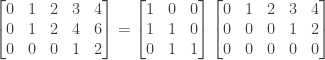
 with unit diagonal and an upper triangular matrix
  .
.
 .
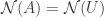
. . The corresponding second and fourth columns of

 and
and  are basic variables with the others being free variables. From the second row above we have
  or
or  . Substituting into the first row we have


 .
. and thus
 .
. we have
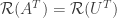
  . The last row of
  is a basis for the (1-dimensional) left nullspace
  such that
  . However we do not need to compute
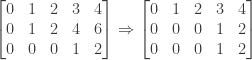


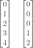
 that they span, find two matrices
  .
.

 . Note that
 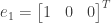 and
and 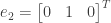 are a basis for
  then for any vector
  in
in  . In particular, we must have
  for the coordinate vectors
  and
and  that form a basis for


 to
to  we must then have
 and that
  and
and 
 .
. . Then we can multiply both sides by
  to produce
  or
or  . But we then have
  so that
  actually exists.
 , the number of columns.
 of
of  is a linear combination of the columns of
  as coefficients. Since the columns of
  . The nullspace
  and since it has dimension
 so that
  .
. . We must have
  or
or
 and
and  . One way to achieve this is to set
  and
and  .
. and
and  . One way to achieve this is to set
  and
and  . We then have

 . The first and third rows of
  .
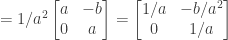
. . We could proceed as we did above, but there is a shortcut: Note that
  so that we are looking for
  . But
. But  and we already have a matrix
  or
or  :
:

 . If
. If  then
then  both a left inverse
  .
.

 ,
,  , and
, and  does
does  ?
? (which is permissible since
 or
or  .
.