Exercise 2.1.7. Of the following, which are subspaces of  ?
?
(a) the set of all sequences that include infinitely many zeros, e.g., 
(b) the set of all sequences of the form  where
where  from some point onward
(c) the set of all decreasing sequences, i.e.,  for all
(d) the set of all sequences such that  converges to a limit as
(e) the set of all arithmetic progressions for which  is constant for all
(f) the set of all geometric progressions of the form  for any choice of
  and
and 
Answer: (a) This set is not a subspace because it is not closed under addition: If we have  and
and  then both
  and
and  are in the set but their sum
  is not.
(b) This set is closed under scalar multiplication: Consider  and suppose for some
  we have
  for
for  . We then have
  . Since we have for we also have
  for . So
  is also a member of the set.
This set is also closed under vector addition. Consider from above and where  and for some we have
  for
for  , and consider the sum
  . Choose
  so that
  and
and  . Then for
  and for so that
  for . The sum
  is therefore also a member of the set.
Since the set is closed under both vector addition and scalar multiplication and it is a subset of the vector space of infinite sequences, it is a subspace of that vector space.
(c) This set is not a subspace because it is not closed under scalar multiplication: The sequence  is a member of the set, but
  is not.
(d) We first check that the set of converging sequences is closed under scalar multiplication. Let be a member of this set, so that  exists. Then for any
  there exists
  such that
  for
for  . Now consider where
  is any scalar. If
  then
then  so that it converges to the limit 0.
Suppose that  and choose any . Since
  exists we can choose such that
  for . Multiplying both sides by
  we have
  . But
. But  . We therefore see that for any we can choose such that
  .
.
This means that  exists and is equal to
  so that for any scalar and converging sequence the sequence is also in the set of converging sequences. Since converges both for and the set is therefore closed under scalar multiplication.
We next check that the set of converging sequences is closed under vector addition. Let also be a member of this set, so that  exists. Then for any there exists such that
  for .
for .
Now consider  and choose any . Since exists we can choose
  such that
  for
for  , and since
  exists we can choose such that
  for . Choose
  such that
  and
and  . Adding both sides of the two inequalities we have
  for
for  .
.
We have  for any
  and
and  , and thus for any we have


So for any we can choose such that  for all . This means that
  exists and is equal to
  so that for any two converging sequences and the sequence is also in the set of converging sequences. The set is therefore closed under vector addition.
Since the set of converging sequences is closed under both vector addition and scalar multiplication and it is a subset of the vector space of infinite sequences, it is a subspace of that vector space.
(e) We first check that the set of arithmetic progressions is closed under scalar multiplication. Let be a member of this set, so that is a constant value for all . Then for  we have
  for all . The sequence is therefore also an arithmetic progression, and the set is closed under scalar multiplication.
We next check that the set of arithmetic progressions is closed under vector addition. Let also be a member of this set, so that  is a constant value for all . Then for
  we have

for all . The sequence is therefore also an arithmetic progression, and the set is closed under vector addition.
Since the set of arithmetic progressions is closed under both vector addition and scalar multiplication and it is a subset of the vector space of infinite sequences, it is a subspace of that vector space.
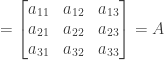
(f) The set of geometric progressions is not a subspace because it is not closed under vector addition: For example, suppose that  (for which
  and
and  ), and
  (for which and
  ). We then have
  . For we have
  (from the first element) and
  (from the second element). If
  is a geometric progression then the third element should be
  instead of the actual value of 13. So is not a geometrical progression for all geometric progressions and , and the set is not closed under vector addition.
UPDATE: Fixed typos in the question ( should have been ) and in the answers to (b) ( should have been ) and (d) (
 should have been ).
UPDATE 2: Fixed typos in the question and answer for (f) (references to  and
and  should have been to , and a reference to should have been to
  ).
).
UPDATE 3: Fixed the answer for (f); the original answer (claiming that  was not a geometric progression) was incorrect. Thanks go to Samuel for pointing this out.
NOTE: This continues a series of posts containing worked out exercises from the (out of print) book Linear Algebra and Its Applications, Third Edition by Gilbert Strang.
If you find these posts useful I encourage you to also check out the more current Linear Algebra and Its Applications, Fourth Edition , Dr Strang’s introductory textbook Introduction to Linear Algebra, Fourth Edition
 and the accompanying free online course, and Dr Strang’s other books
 .
.


 that defines a plane
  in 3-space. For the parallel plane
  through the origin find its equation and explain whether
  must be a solution of the equation for
  satisfies this criterion and its plane
  will not be.
  and
and  for any vector
  ).
).

 for all
 for all

 such that it adds an extra one to each component, e.g.,
 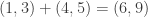 instead of
  . Assume the rule for scalar multiplication is left unchanged. Which of the above rules is broken by this redefinition of addition?
 and define scalar multiplication on the same set so that
  . Show that the set of positive real numbers is a vector space under the operations thus defined, and describe the zero vector.
 and
and  rule 1 is satisfied:


 as the zero vector:
 :
:


 we have


 we have

 and
and  to denote the following definitions of vector addition and scalar multiplication on the set of positive real numbers:
 and
and 


 as
as 


 where
where  is a 3 by 3 symmetric matrix and
  is a 3 by 3 lower triangular matrix. Now, in general symmetric matrices can have nonzero entries above the diagonal, to match corresponding nonzero entries below the diagonal. Therefore in general the sum
 ,
,  , and
, and  (the entries of
  ,
,  , and
, and  from
from 

 ,
,  , and
, and  .
.


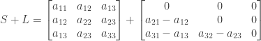
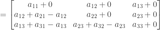
 . Put another way, adding 3 by 3 symmetric matrices and 3 by 3 lower triangular matrices together can produce any possible 3 by 3 matrix. So the smallest possible subspace containing both all 3 x 3 symmetric matrices and all 3 by 3 lower triangular matrices is the space of all 3 by 3 matrices.
 for
for  . If
. If  for all
  . So we have
  and
and  is a diagonal matrix and
  is also a diagonal matrix (even if
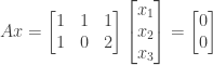
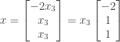
 is therefore the x axis, i.e., the set of vectors of the form
  .
.
 or
or  . The nullspace
  passing through the origin at a 45 degree angle to the x axis.
 the column space
  contains all vectors of the form
 .
. we have
 .
. to be 2 by 1 rather than 3 by 1. Thanks go to James Teow for catching the error.
 with the first component
 with the first component
 for which

 and
and 
 for which
 and
and  the sum
  is also in the set. It is also closed under scalar multiplication, since for any vector
  is also in the set.
 the product
  is not in the set. It is also not closed under vector addition, since for the vectors
  and
and  is not in the set.
 and
and  are in the set but their sum
  .
. the product
  is also a linear combination of
  their sum
  is also a linear combination of
  in the set, for the scalar product
  we have
 we have
 where
where  ,
,  , etc. This set is closed under vector addition, since the sum or difference of two integers is always an integer. However it is not closed under scalar multiplication, since (for example) multiplying
  produces a result
  not in the set.
 , is closed under scalar multiplication but not under vector addition.
 . We have
  where
where  is the 2 by 2 identity matrix, and thus
  . So we have
 where
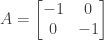
where  . By experiment we see that the following matrix will work

 to
to  and in general would send the vector
  to
to  . By experiment we see that the matrix
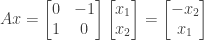
 and in general would send the vector
  . By experiment we see that the matrix