Review exercise 1.27. State whether the following are true or false. If true explain why, and if false provide a counterexample.
(1) If a matrix  can be factored as
 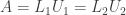 where
where  and
and  are lower triangular with unit diagonals and
  and
and  are upper triangular, then
  and
and  . (In other words, the factorization
  is unique.)
(2) If for a matrix we have  then is invertible and
  .
.
(3) If all the diagonal entries of a matrix are zero then is singular.
Answer: (1) True. Since and are lower triangular with unit diagonal both matrices are invertible, and their inverses are also lower triangular with unit diagonal. (See the proof of this below at the end of the post.) Similarly since and are upper triangular with nonzero diagonal those matrices are invertible as well, and their inverses are also upper triangular with nonzero diagonal.
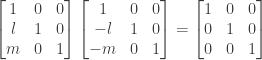
We then start with the equation  and multiply both sides by
  on the left and by
  on the right:

This equation reduces to  where
where  is the product matrix. Now since is the product of two lower triangular matrices with unit diagonal (i.e., and ), it itself is a lower triangular matrix with unit diagonal. Since is the product of two upper triangular matrices (i.e., and ), it is also an upper triangular matrix. Since is both lower triangular and upper triangular it must be a diagonal matrix, and since its diagonal entries are all 1 we must have
  .
.
Since  we can multiply both sides on the left by to obtain
 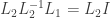 or . Similarly since
  we can multiply both sides on the right by to obtain
  or
or  . So the factorization is unique.
(2) True. Assume . We have 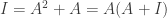 so that
  is a right inverse for . We also have
 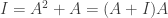 so that is a left inverse for . Since
  is both a left and right inverse of we know that is invertible and that .
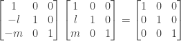
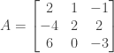
(3) False. The matrix

has zeros on the diagonal but is nonsingular. In fact we have

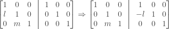
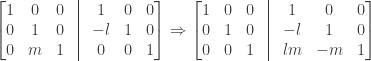
Proof of the result used in (1) above: Assume  is a lower triangular matrix with unit diagonal. That is invertible can be seen from Gauss-Jordan elimination (here shown in a 4 by 4 example, although the argument generalizes to all
  ):
):

Note that in forward elimination each of the diagonal entries of will remain as is, since each of these entries has only zeros above it; each of the zero entries above the diagonal will remain unchanged as well, for the same reason. When forward elimination completes the left hand matrix will be the identity matrix since it will have zeros below the diagonal (from forward elimination), ones on the diagonal (as noted above), and zeroes above the diagonal (also as noted above). Gauss-Jordan elimination is thus guaranteed to complete successfully, so is invertible.
The right-hand matrix at the end of Gauss-Jordan elimination will be the inverse of . That matrix was produced from the identity matrix by forward elimination only, since backward elimination was not necessary. For the same reason noted above for the left-hand matrix, forward elimination will preserve the unit diagonal in the right-hand matrix and the zeros above it, with the only possible non-zero entries occurring below the unit diagonal. We thus see that if is a lower-triangular matrix with unit diagonal then it is invertible and its inverse  is also a lower-triangular matrix with unit diagonal.
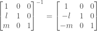
Assume  is an upper triangular matrix with nonzero diagonal. That is invertible can be seen from Gauss-Jordan elimination (again shown in a 4 by 4 example):

Note that forward elimination is not necessary: There are nonzero entries on the diagonal and zeros below them, so we have pivots in every column; therefore the left-hand matrix is nonsingular and is guaranteed to have an inverse.
We can find that inverse by doing backward elimination to eliminate the entries above the diagonal in the left-hand matrix, and then dividing by the pivots. Note that since backward elimination starts with all zero entries below the diagonal in the right-hand matrix, it will not produce any nonzero entries below the diagonal in that matrix. Also, the diagonal entries in the right-hand matrix are not affected by backward elimination, for the same reason. After backward elimination completes the diagonal entries in the right-hand matrix will still be ones, and any nonzero entries produced will be above the diagonal. Dividing by the pivots in the left-hand matrix will then produce nonzero entries in the diagonal of the right-hand matrix.
The final right-hand matrix after completion of Gauss-Jordan elimination will therefore be an upper triangular matrix with nonzero diagonal entries. We thus see that if is an upper-triangular matrix with nonzero diagonal then it is invertible and its inverse  is also an upper-triangular matrix with nonzero diagonal.
NOTE: This continues a series of posts containing worked out exercises from the (out of print) book Linear Algebra and Its Applications, Third Edition by Gilbert Strang.
If you find these posts useful I encourage you to also check out the more current Linear Algebra and Its Applications, Fourth Edition , Dr Strang’s introductory textbook Introduction to Linear Algebra, Fourth Edition
 and the accompanying free online course, and Dr Strang’s other books
 .
.


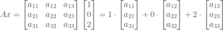
 would make the product
  have 1 times column 1 of A plus 2 times column 3?


 and
and  position will also produce zeros in the
  and
and  positions, so that there is no possible pivot in column 3.
 . Since
  to determine that 5 times row 2 was subtracted from row 3 in elimination.
 we know that
  so
so  where
where  we see that the pivots (i.e., the diagonal entries of D) are all 1.
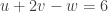 defines a plane in 3-space. Find equations that define the following:
 and
and 

 . The equation
  satisfies this condition, and produces a plane parallel to the original plane.
 . Therefore if we take the equation for the original plane and change the term involving
  we can produce a new and different equation corresponding to a new plane containing these points. One such equation is
  .
. and
and  . One such equation is
  . Since the point
  and
and 

 .
.


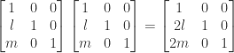
 . Then for

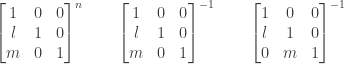
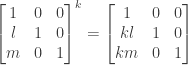
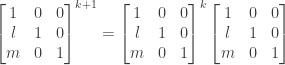
 for any matrix
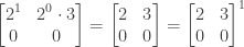

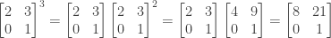
 entry of each matrix appears to be
  in general, but the
  entry is more complicated. The expression
  looks as if it might work; for
 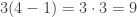 and for
  .
.


 we have
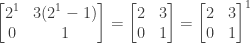
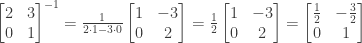

 also have an inverse? If so, what is it?
 ?
? .
. and therefore
  . But
. But  so we have
  and
and  is a left inverse for
  and therefore
  . But
. But  so we have
  and
and  .
. . If
. If  . Since
  we see that
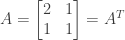


 and the columns of
  .
. to produce
 for all matrices P in the group?
 .
. choices for where to put the 1 entry in row 2,
  choices for where to put the 1 entry in row 3, and so on until we have only 1 choice for where to put the 1 entry in row
  .
. or six 3 by 3 permutation matrices, of which one is the identity matrix
  for which
  for any
  .
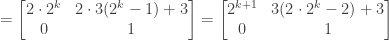
. . We then also have
  and in general
  . We then have
  , and in general
  is the smallest
  .
. and
and 


 . Substituting
  and
and  . The solution is therefore

