Review exercise 1.12. State whether the following are true or false. If a statement is true explain why it is true. If a statement is false provide a counter-example.
(a) If  is invertible and
  has the same rows as but in reverse order, then is invertible as well.
(b) If and are both symmetric matrices then their product  is also a symmetric matrix.
(c) If and are both invertible then their product  is also invertible.
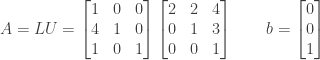
(d) If is a nonsingular matrix then it can be factored into the product  of a lower triangular and upper triangular matrix.
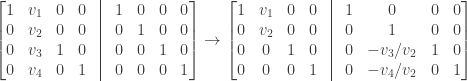
Answer: (a) True. If has the same rows as but in reverse order then we have  where
where  is the permutation matrix that reverses the order of rows. For example, for the 3 by 3 case we have

If we apply twice then it restores the order of the rows back to the original order; in other words  so that
  .
.
If is invertible then  exists. Consider the product
  . We have

so that is a right inverse for . We also have

so that is a left inverse for as well. Since is both a left and right inverse for we have  so that is invertible if is.
Incidentally, note that while multiplying by on the left reverses the order of the rows, multiplying by on the right reverse the order of the columns. For example, in the 3 by 3 case we have

Thus if exists and then exists and consists of with its columns reversed.
(b) False. The product of two symmetric matrices is not necessarily itself a symmetric matrix, as shown by the following counterexample:

(c) True. Suppose that both and are invertible; then both and  exist. Consider the product matrices and
  . We have

and also

So  is both a left and right inverse for and thus
 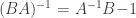 . If both and are invertible then their product is also.
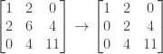
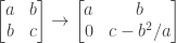
(d) False. A matrix cannot necessarily be factored into the form because you may need to do row exchanges in order for elimination to succeed. Consider the following counterexample:
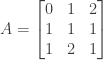
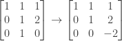
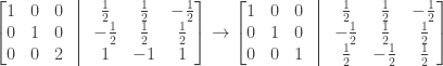
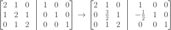
This matrix requires exchanging the first and second rows before elimination can commence. We can do this by multiplying by an appropriate permutation matrix:

We then multiply the (new) first row by 1 and subtract it from the third row (i.e., the multiplier  ):
):

and then multiply the second row by 1 and subtract it from the third ( ):
):
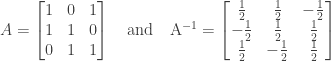
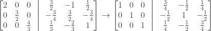
We then have

and

So a matrix cannot always be factored into the form .
NOTE: This continues a series of posts containing worked out exercises from the (out of print) book Linear Algebra and Its Applications, Third Edition by Gilbert Strang.
If you find these posts useful I encourage you to also check out the more current Linear Algebra and Its Applications, Fourth Edition , Dr Strang’s introductory textbook Introduction to Linear Algebra, Fourth Edition
 and the accompanying free online course, and Dr Strang’s other books
 .
.


 .
. ):
):
 ):
):


 times the first row from the second row (
 ):
):


 be for the system to have no solution? One solution? An infinite number of solutions?
 then the system reduces to
 and
and  is (obviously) a solution.
 then we can multiply the first equation by
  and subtract it from the second equation to obtain the following system:
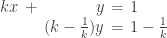
 then this reduces to
 for which
  .
. then we can solve for
  as follows:

 as follows:


 . For example, for
  the unique solution is
 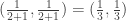 .
. which matches that given by our formula:
 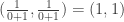 .
.  , for which the solution
 .
. by
by 
 ?
? we must have


 we obtain
  or
or  so that
  .
.

 so that we can choose

 so that we can choose


 and
and  to find a solution to

 and
and  we have
  also. Since
  we have
  so that

 and
and  we have
  . We then have
  so that
  and
and
 is equal to the last column of the 3 by 3 identity matrix
  . Since
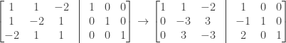
  is a 2 by 2 matrix that adds the first equation of a linear system to the second equation. What is
  ?
?  ?
?  ?
?
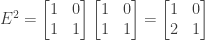


 we have
 we have
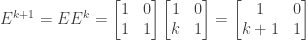

 we have


 and subtracting it from the second row, and multiplying the third row by
  and subtracting it from the first row:
 and subtract it from the third row:
 and subtracting it from the second row:
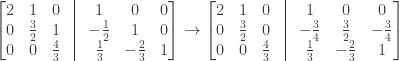

 , and the third row by
  :
:


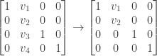
 where
where
 where
where  .
.
