Exercise 1.7.10. When partial pivoting is used show that  for all multipliers
  in
in  . In addition, show that if
  for all
  and
and  then after producing zeros in the first column we have
  , and in general we have
  after producing zeros in column
  . Finally, show an 3 by 3 matrix with and for which the last pivot is 4.
Answer: (a) With partial pivoting we choose the pivot  for each row and column in turn so that the pivot is the largest (in absolute value) of all the candidate pivots in the same column. Thus
  where
where  are all the other candidate pivots. The multipliers are then equal to the candidate pivots divided by the chosen pivot, so that
  . But since we have
  .
.
(b) Assume that  for all and . Without loss of generality assume that
  for all
  . (If this were not true then we could simply employ partial pivoting and do a row exchange to ensure that this would be the case.) Also assume that
  (i.e., the matrix is not singular). We then have
  for and thus
 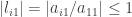 for .
for .
Let  be the matrix produced after the first stage of elimination. Then for
  we have
  and thus
  and thus
  . For we have
 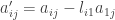 so that
  for . But we have for all (and thus
  ) and
) and  for . Thus for the product
  we have
  for and for the difference
  we have
  for (with the maximum difference occurring when
  and
and  or vice versa).
So we have for and we also have  for . For the matrix after the first stage of elimination we therefore have
  for all and .
Assume that after stage of elimination we have produced the matrix  with
with  for all and and consider stage
  of elimination. In this stage our goal is to find an appropriate pivot for column and produce zeros in column for all rows below . Without loss of generality assume that
  for all
  (otherwise we can do a row exchange as noted above). Also assume that
  (i.e., the matrix is not singular). We then have
  for and thus
  for .
for .
Let  be the matrix produced after stage of elimination. Then for
  we have
  and thus
  and thus
  . For we have
 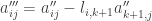 so that
  for . But we have for all (and thus
  ) and
) and  for . Thus for the product
  we have
 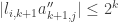 for and for the difference
  we have
 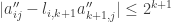 for (with the maximum difference occurring when
  and
and  or vice versa).
So we have  for and we also have
  for . For the matrix after stage of elimination (which produces zeros in column ) we therefore have
  for all and . For
  we also have
  for all and after the first stage of elimination (which produces zeros in column 1). Therefore by induction if in the original matrix
  we have then for all
  if we do elimination with partial pivoting then after stage of elimination (which produces zeros in column ) we will have a matrix for which
  .
.
(c) One way to construct the requested matrix is to start with the desired end result and work backward to find a matrix for which elimination will produce that result, assuming that the absolute value of the multiplier at each step is 1 (the largest absolute value allowed under our assumption) and that after stage we have no value larger in absolute value than  .
.
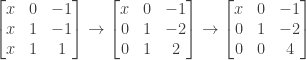
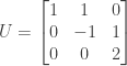
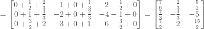
Thus in the final matrix (after stage 2 of elimination) we assume we have a pivot of 4 in column 3 but as yet unknown values for the other entries. The successive matrices at the various stages of elimination (the original matrix and the matrices after stage 1 and stage 2) would then be as follows:

We assume a multiplier of  for the single elimination step in stage 2, and prior to that step (i.e., after stage 1 of elimination) we can have no entry larger in absolute value than 2. The successive matrices at the various stages of elimination would then be as follows:

so that subtracting row 2 from row 3 in stage 2 (i.e., using the multiplier ) would produce the value 4 in the pivot position.
We now need to figure out how to produce a value of 2 in the  position and a value of -2 in the
  position after stage 1 of elimination. Stage 1 consists of two elimination steps, and we assume a multiplier of 1 or -1 for each step; also, all entries in the original matrix can have an absolute value no greater than 1. The original matrix prior to stage 1 of elimination can then be as follows:

with the multiplier  and the multiplier
  (i.e., in stage 1 of elimination we are adding row 1 to row 2 and subtracting row 1 from row 3).
Now that we have picked entries for column 3 in the original matrix and suitable multipliers for all elimination steps, we need to pick entries for column 1 and column 2 of the original matrix that are consistent with the chosen multipliers and ensure that elimination will produce nonzero pivots in columns 1 and 2.
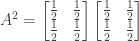
We first pick values for the  and entries in the matrix after stage 1 of elimination; since we are using the multiplier those entries should be the same in order to produce a zero in the position after stage 2. We’ll try picking a value of 1 for both entries:

From above we know that in stage 1 of elimination row 1 is added to row 2 (i.e., the multiplier ) and row 1 is subtracted from row 3 (i.e., the multiplier ). Since we have to end up with the same value in the and  positions in either case, the easiest approach is to assume that the
  position in the original matrix has a zero entry, so that adding or subtracting it doesn’t change the preexisting entries for rows 2 and 3:
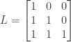
Finally, we need entries in the first column such that adding row 1 to row 2 and subtracting row 1 from row 3 will produce zero:

This completes our task. We now have a matrix

for which and , and for which elimination produces a final pivot of 4.
NOTE: This continues a series of posts containing worked out exercises from the (out of print) book Linear Algebra and Its Applications, Third Edition by Gilbert Strang.
If you find these posts useful I encourage you to also check out the more current Linear Algebra and Its Applications, Fourth Edition , Dr Strang’s introductory textbook Introduction to Linear Algebra, Fourth Edition
 and the accompanying free online course, and Dr Strang’s other books
 .
.


 , which is zero for all these matrices.


 possible matrices of this type. At present I don’t know of a good method to determine whether the majority of those matrices are invertible or not. I’ll update this post later if and when I have time to work on this some more.
 or
or  .
.


 ).
).


 ).
).


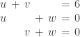
 into the second equation to obtain
 into the first equation to obtain


 , and back-substituting the value of
  . Finally, back-substituting the value of
  . The solution is therefore


 and (a)
  , (b)
, (b)  , and (c)
  .
.
 , we have
  . Then
  or
or  . Substituting for
  we then have
  or
or  . So we can freely choose
  and then that value determines the values of
  and
and  then
then


 then
then
 then
then
 .
.

 we have
  . We choose
  . Since
 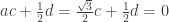 we have
  . Finally, since
  we have
  or
or  . We choose
  .
.
 in this case so that we also have
  , and
, and  .
. then
then

 then since
  we have
  . Since
  we again have
  (and also

 we have
  or
or  . Since
  we have
  . Thus we can choose any value for
  and
and  . We then have

 and
and 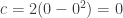 . We then have

 and
and  . We then have

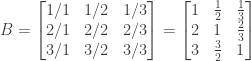
 as follows
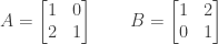
 and
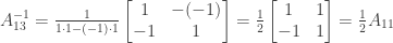
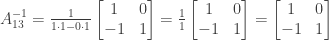
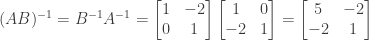
and  , the inverses
  ,
,  , and
, and  .
.


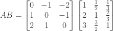
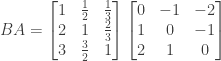
 and
and  .
. of the above matrices.


 and
and  . This follows from equation 1M(i) in section 1.6:
  .)
.)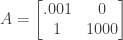
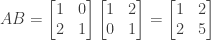
 (1/.001) to multiply the first row and subtract it from the second:

 (.001/1) to multiply the first row and subtract it from the second:

