
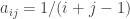
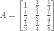
Exercise 1.7.8. Take the 10 by 10 Hilbert matrix 


Answer: We can use the open source statistics software R for this exercise. The following R commands will define a 10 by 10 Hilbert matrix. The first command defines 
> A <- array(0, dim=c(10,10))
> for (i in 1:10) {for (j in 1:10) {A[i, j] <- 1/(i+j-1)}}
>
We then print the matrix to double-check that it appears to be correct (we use the option() function to limit the number of digits printed per entry and increase the width of the printable area, so that the entire matrix can be displayed more compactly):
> options(digits=3)
> options(width=90)
> A
[,1] [,2] [,3] [,4] [,5] [,6] [,7] [,8] [,9] [,10]
[1,] 1.000 0.500 0.3333 0.2500 0.2000 0.1667 0.1429 0.1250 0.1111 0.1000
[2,] 0.500 0.333 0.2500 0.2000 0.1667 0.1429 0.1250 0.1111 0.1000 0.0909
[3,] 0.333 0.250 0.2000 0.1667 0.1429 0.1250 0.1111 0.1000 0.0909 0.0833
[4,] 0.250 0.200 0.1667 0.1429 0.1250 0.1111 0.1000 0.0909 0.0833 0.0769
[5,] 0.200 0.167 0.1429 0.1250 0.1111 0.1000 0.0909 0.0833 0.0769 0.0714
[6,] 0.167 0.143 0.1250 0.1111 0.1000 0.0909 0.0833 0.0769 0.0714 0.0667
[7,] 0.143 0.125 0.1111 0.1000 0.0909 0.0833 0.0769 0.0714 0.0667 0.0625
[8,] 0.125 0.111 0.1000 0.0909 0.0833 0.0769 0.0714 0.0667 0.0625 0.0588
[9,] 0.111 0.100 0.0909 0.0833 0.0769 0.0714 0.0667 0.0625 0.0588 0.0556
[10,] 0.100 0.091 0.0833 0.0769 0.0714 0.0667 0.0625 0.0588 0.0556 0.0526
>
We next define 
> b <- array(0, dim=c(10))
> b[1] <- 1
> b
 [1] 1 0 0 0 0 0 0 0 0 0
>
We can now use the R solve() function to solve for
> x <- solve(A, b)
> x
[1]      100    -4950    79195  -600553  2522294 -6305679  9608580 -8750614  4375282
[10]  -923666
>
We then multiply 
> A %*% x
           [,1]
 [1,]  1.00e+00
 [2,] -1.89e-10
 [3,] -2.04e-10
 [4,] -1.60e-10
 [5,] -1.02e-10
 [6,]  3.64e-11
 [7,]  2.18e-11
 [8,]  7.28e-11
 [9,]  0.00e+00
[10,]  0.00e+00
>
Finally we tweak
> b2 <- b
> b2[10] <- .01
> b2
[1] 1.00 0.00 0.00 0.00 0.00 0.00 0.00 0.00 0.00 0.01
> x2 <- solve(A, b2)
> x2
[1] -9.14e+03  8.26e+05 -1.82e+07  1.70e+08 -8.30e+08  2.32e+09 -3.87e+09  3.80e+09
[9] -2.02e+09  4.48e+08
>
Note that the very minor change to
NOTE: This continues a series of posts containing worked out exercises from the (out of print) book Linear Algebra and Its Applications, Third Edition by Gilbert Strang.
If you find these posts useful I encourage you to also check out the more current Linear Algebra and Its Applications, Fourth Edition, Dr Strang’s introductory textbook Introduction to Linear Algebra, Fourth Edition
and the accompanying free online course, and Dr Strang’s other books
.
 and
and  are solutions to
 and subtract it from the second row, and then multiply the first row times
  and subtract it from the third row:


 and
and  (instead of
  and
and 
 this equation would become
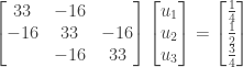
![\rightarrow -u_2 + 2u_1 = h^2 f(jh) + 1 = h^2 [f(jh) + \frac{1}{h^2}]](https://s0.wp.com/latex.php?latex=%5Crightarrow+-u_2+%2B+2u_1+%3D+h%5E2+f%28jh%29+%2B+1+%3D+h%5E2+%5Bf%28jh%29+%2B+%5Cfrac%7B1%7D%7Bh%5E2%7D%5D&bg=ffffff&fg=333333&s=0&c=20201002)
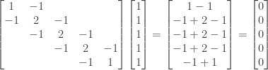
 the corresponding 5 by 5 finite-difference matrix is then
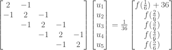
 the corresponding difference equation is
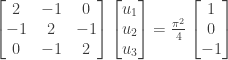
 . Solve the above equation for
  and compare their values to the true solution
  at
at  ,
,  and
and  .
.
 we have
 we have
 :
:
 we have


 by
by  (and hence
  ) and the boundary condition
  by
by  (and hence
  ).
). yields zero. Similarly, show that for any solution
  to the original differential equation,
  is also a solution.
 in finite difference terms as
![- [u_{j-1} - 2u_j + u_j+1]/h^2 = f(jh)](https://s0.wp.com/latex.php?latex=-+%5Bu_%7Bj-1%7D+-+2u_j+%2B+u_j%2B1%5D%2Fh%5E2+%3D+f%28jh%29&bg=ffffff&fg=333333&s=0&c=20201002)

 . The above equation can then be rewritten as
 is the approximation of
  .
.
 the above equation becomes
 ,
,  , and
, and  . Since

 . Then we have
![-\frac{d^2v}{dx^2} = -\frac{d^2}{dx^2} [u(x) + 1] = -\frac{d^2}{dx^2}u(x) - \frac{d^2}{dx^2}(1)](https://s0.wp.com/latex.php?latex=-%5Cfrac%7Bd%5E2v%7D%7Bdx%5E2%7D+%3D+-%5Cfrac%7Bd%5E2%7D%7Bdx%5E2%7D+%5Bu%28x%29+%2B+1%5D+%3D+-%5Cfrac%7Bd%5E2%7D%7Bdx%5E2%7Du%28x%29+-+%5Cfrac%7Bd%5E2%7D%7Bdx%5E2%7D%281%29&bg=ffffff&fg=333333&s=0&c=20201002)

![\frac{dv}{dx}(0) = \frac{d}{dx}[u(0) + 1] = \frac{d}{dx}u(o) + \frac{d}{dx}(1) = \frac{du}{dx}(o) + 0 = \frac{du}{dx}(o) = 0](https://s0.wp.com/latex.php?latex=%5Cfrac%7Bdv%7D%7Bdx%7D%280%29+%3D+%5Cfrac%7Bd%7D%7Bdx%7D%5Bu%280%29+%2B+1%5D+%3D+%5Cfrac%7Bd%7D%7Bdx%7Du%28o%29+%2B+%5Cfrac%7Bd%7D%7Bdx%7D%281%29+%3D+%5Cfrac%7Bdu%7D%7Bdx%7D%28o%29+%2B+0+%3D+%5Cfrac%7Bdu%7D%7Bdx%7D%28o%29+%3D+0&bg=ffffff&fg=333333&s=0&c=20201002)
![\frac{dv}{dx}(1) = \frac{d}{dx}[u(1) + 1] = \frac{d}{dx}u(1) + \frac{d}{dx}(1) = \frac{du}{dx}(1) + 0 = \frac{du}{dx}(1) = 0](https://s0.wp.com/latex.php?latex=%5Cfrac%7Bdv%7D%7Bdx%7D%281%29+%3D+%5Cfrac%7Bd%7D%7Bdx%7D%5Bu%281%29+%2B+1%5D+%3D+%5Cfrac%7Bd%7D%7Bdx%7Du%281%29+%2B+%5Cfrac%7Bd%7D%7Bdx%7D%281%29+%3D+%5Cfrac%7Bdu%7D%7Bdx%7D%281%29+%2B+0+%3D+%5Cfrac%7Bdu%7D%7Bdx%7D%281%29+%3D+0&bg=ffffff&fg=333333&s=0&c=20201002)

![-\frac{d^2u}{dx^2} + u \approx - [u(x-h) - 2u(x) + u(x+h)]/h^2 + u(x)](https://s0.wp.com/latex.php?latex=-%5Cfrac%7Bd%5E2u%7D%7Bdx%5E2%7D+%2B+u+%5Capprox+-+%5Bu%28x-h%29+-+2u%28x%29+%2B+u%28x%2Bh%29%5D%2Fh%5E2+%2B+u%28x%29&bg=ffffff&fg=333333&s=0&c=20201002)
![-[u_{j-1} - 2u_j + u_{j+1} + u_j]/h^2 + u_j = jh](https://s0.wp.com/latex.php?latex=-%5Bu_%7Bj-1%7D+-+2u_j+%2B+u_%7Bj%2B1%7D+%2B+u_j%5D%2Fh%5E2+%2B+u_j+%3D+jh&bg=ffffff&fg=333333&s=0&c=20201002)


 . The above equation can then be rewritten as


 so that we have
  . For
. For 


 instead of
  .)
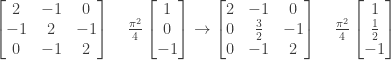
.) and subtract it from the second row:
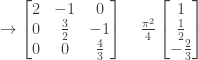
 and subtract it from the third row:
 and subtract it from the fourth row:
 and subtract it from the fifth row:
 are square matrices, and that
  is invertible. Show that
  is invertible as well. (Use the fact that
  .)
.) and
and  exist and have the same number of rows and columns. We then have


![\rightarrow [A(I - BA)^{-1} B + I] (I - AB) = AB - AB + I = I](https://s0.wp.com/latex.php?latex=%5Crightarrow+%5BA%28I+-+BA%29%5E%7B-1%7D+B+%2B+I%5D+%28I+-+AB%29+%3D+AB+-+AB+%2B+I+%3D+I&bg=ffffff&fg=333333&s=0&c=20201002)
 is a left inverse for
 ![(I - AB)[A(I - BA)^{-1} B + I]](https://s0.wp.com/latex.php?latex=%28I+-+AB%29%5BA%28I+-+BA%29%5E%7B-1%7D+B+%2B+I%5D&bg=ffffff&fg=333333&s=0&c=20201002)


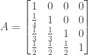
 and subtracting it from the second row, multiplying the first row by the multiplier


