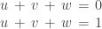
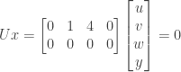
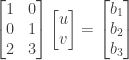
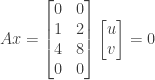
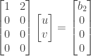
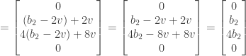
Exercise 2.2.4. Consider the system of linear equations represented by the following matrix:

Find the echelon matrix  , a set of basic variables, a set of free variables, and the general solution to
  . Then use elimination to find when the system
  has a solution, and express that solution as the sum of a particular solution and the general solution to . Finally, find the rank of
  .
.
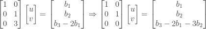
Answer: We perform elimination on by subtracting 2 times the first row from the second row (i.e., using the multiplier  ):
):

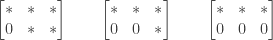
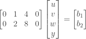
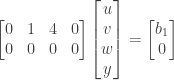
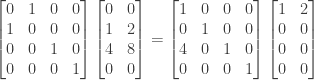
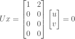
This completes elimination, and leaves us with the echelon matrix

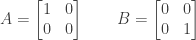
and the factorization  :
:
We now solve for

which is equivalent to
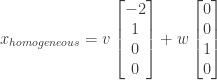
The pivot in is in column 2, so the (only) basic variable is  and the free variables are
  ,
,  and
and  .
.
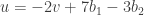
From the first row of we have  and thus
  . We then have

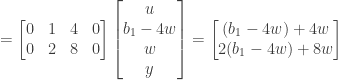
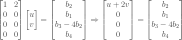
In considering the inhomogeneous system or
the elimination sequence above would produce the system  or
or

From the second equation we must have  or
or  . Thus for to have a solution the vector
  must lie on the line passing through the origin and the point
  so that
  .
.
Taking  produces the system

which after elimination becomes
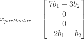
The first equation gives  or
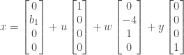
or  . Setting the free variables , , and all to zero produces the particular solution
  to the system
We can combine the particular solution to this system with the solution to to produce the general solution for the system
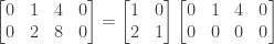
We can check this solution as follows:


The rank of is 1, the number of basic variables (or pivots).
UPDATE: I expanded the answer to conform to the presentation in the answer to exercise 2.2.5.
UPDATE 2: I corrected the value for used in various places. Thanks go to Zoi for catching this error!
NOTE: This continues a series of posts containing worked out exercises from the (out of print) book Linear Algebra and Its Applications, Third Edition by Gilbert Strang.
If you find these posts useful I encourage you to also check out the more current Linear Algebra and Its Applications, Fourth Edition , Dr Strang’s introductory textbook Introduction to Linear Algebra, Fourth Edition
 and the accompanying free online course, and Dr Strang’s other books
 .
.


 does this system have a solution?
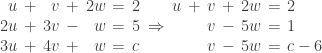

 or
or  .
.

 in order for the system to have a solution. The matrix
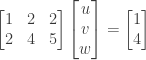


 or
or 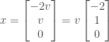

 . Substituting into the first equation and setting the free variable
  or
or  . The particular solution is thus
  .
. for the system
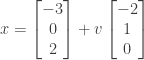

 as follows:
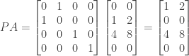
 by subtracting 4 times the first row from the third row (i.e., using the multiplier
  ):
):

 :
:


 . From the third equation we must have
  or
or  . Thus for
  .
. produces the system
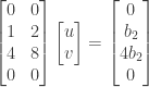
 or
or  . Setting the free variable
 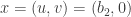 to the system


 ):
):


 and thus
  . From the first row of
  and can substitute for
  or
or  . We then have
 ) always have solutions. To find a system with no solution we therefore have to look at systems of two equations and three unknowns. For example, the system