
Exercise 2.3.5. If we test vectors by independence by putting them into the rows of a matrix (rather than the columns), how can we determine whether or not the rows are independent using the elimination process? Determine the independence of the vectors in exercise 2.3.1 using this method.
Answer: My goal in this post is to (as much as possible) answer the question using the material introduced in section 2.3 and prior sections of the book. The material in section 2.4, in particular regarding the relationship of the row space to the column space, can simplify the answer, or at least make it more rigorous.
Assume that we have a set of 


The first thing to note is that if 
The next thing to note is that if any of the rows of the matrix is initially zero then again the row vectors must be linearly dependent, since we can multiply that row by a nonzero weight and all other rows by zero to produce a nontrivial linear combination of the rows that is equal to the zero vector.
If the number of rows 
Suppose at some point in the elimination process a row of all zero values is produced. Since the multipliers in Gaussian elimination are nonzero, the zero row is a linear combination of the original row vectors in which at least one of the weights is nonzero. (For example, if the first entry in the original row vector were nonzero then the first row would be included in the linear combination with weight equal to the negative of the multiplier used to produce a zero in the first position of the row.) Again we have a nontrivial linear combination of rows equaling the zero vector, and thus the rows are linearly dependent.
On the other hand, suppose elimination completes and produces an echelon matrix with no zero rows, i.e., every row has a pivot. The row vectors in this matrix are then linearly independent, as we can see by looking at the pivots:
Start with the pivot in the the first row of the echelon matrix. Since this value is a pivot there are zeros below it, and since this is the first row the pivot is the only nonzero value in this column for any of the rows. Any linear combination of the row vectors that equals zero must therefore multiply the first row by zero. Similarly the pivot in the second row has zeros below it, and since the first row was multiplied by zero it is now the only nonzero value that can contribute to the linear combination. For a linear combination of the rows to equal zero we must therefore also multiply the second row by zero.
Since every row of the echelon matrix has a pivot, looking at each row in turn we can see that for a linear combination of the rows to equal zero we must multiply each row of the echelon matrix by zero. This implies that the rows of the echelon matrix are linearly independent.
What about the rows of the original matrix? If the rows of the echelon matrix are independent were the original rows independent as well? The answer is yes, as can be seen by looking at the spaces spanned by the rows in each case:
The initial set of row vectors spans a vector space; since each row vector has
Performing Gaussian elimination on the matrix takes the initial set of row vectors and at each step replaces one row with a linear combination of that row and another row. More specifically, a given elimination step takes a row vector 


Although each elimination step produces a new set of row vectors (since one row is replaced with a new one as described above) that new set spans the exact same space as the original row. To see this, suppose 


Now suppose we replace


Since 

Now consider a vector 

In reversing the elimination step we replace 


Since
Combined with the previous result we thus conclude that each elimination step does not change the space spanned by the row vectors. The space spanned by the initial set of row vectors is thus exactly the same as the space spanned by the row vectors of the echelon matrix produced by elimination.
If the 


We conclude that if the set of
We now apply the above discussion to the vectors of exercise 2.3.1:

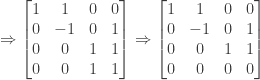
We form a matrix containing as rows the vectors above, and then perform Gaussian elimination on this matrix:

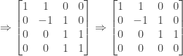
Since the echelon matrix produced by elimination has a row of zeros its row vectors are linearly dependent, and thus the initial set of row vectors is linearly dependent as well.
NOTE: This continues a series of posts containing worked out exercises from the (out of print) book Linear Algebra and Its Applications, Third Edition by Gilbert Strang.
If you find these posts useful I encourage you to also check out the more current Linear Algebra and Its Applications, Fourth Edition, Dr Strang’s introductory textbook Introduction to Linear Algebra, Fourth Edition
and the accompanying free online course, and Dr Strang’s other books
.
 ,
,  , and
, and  are linearly independent. (The book says
  ,
,  , and
, and  also linearly independent?
 ,
,  , and
, and  with weights
  ,
,  , and
, and  . We have

 ,
,  , and
, and  .
.


 or
or  ,
,  or
or  , and
, and  or
or  .
. only if
 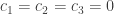 we see that
 are linearly dependent if any of the diagonal entries
  ,
,  , or
, or  is zero.
 whose columns are the rows of
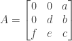

 we have the following matrix:
 . So if
  we have the following matrix
 we have the following matrix
 ,
,  , and
, and 
 , the vectors
  ,
,  ,
,  , and
, and 
 ,
,  , and
, and  , the vectors
  ,
,  ,
,  , and
, and 

 the columns (and thus the vectors in question) are linearly independent.
 ) we have

 must be linearly dependent, so the four vectors in question are always linearly dependent for any values of
  . Also, solve
  to determine whether the vectors span
  .
.


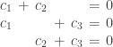
 is a free variable and
  , from the third equation we have
  or
or  . From the second equation we have
  or
or  . Finally, from the first equation we have
  . This means that we have
  and thus the vectors are not linearly independent. More specifically, we can express
  .
.
 . Thus this system has no solution, and we conclude that the vectors in question do not span
  where
where  and
and  ; for example
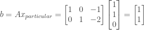
 as a solution, but the general system has no particular solution since
  for any
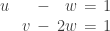
  not be equal to each other. For example, consider the system


 ?
?

 is the only variable referenced in the homogeneous solution it must be the only free variable, with
  and
and  must therefore have the form
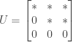
 because we need to account for the particular condition
  that is required for the system
  resulting from the elimination operations applied to
 or
or  ). We then have to do elimination operations only for the third row, and those operations will produce the third element of
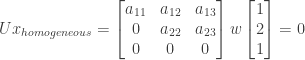
 and so adds no new information. We can therefore follow the same process as in exercise 2.2.12 to find values for the first two rows of
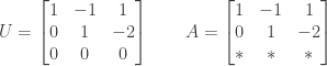


 as the last element of
  or
or  . The second operation means we must have
 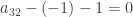 or
or  as well as
  or
or  . The proposed value for
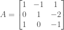


 . If this were not the case then the system would have no solution.

 and
and  are nonzero (because they are pivots).
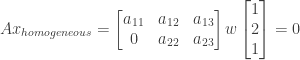


 . We can then satisfy the first equation by assigning
  and
and  . The pivot
  as well. We can then satisfy the second equation by assigning
  . Our proposed value of
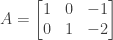


 be a system of
  . In this case what is the rank of
  .
.
 ?
? and
and  and the free variables are
  and
and  .
. or
or  . Substituting the value of
  or
or  . The solution to
  can then be expressed in terms of the free variables
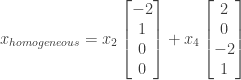

 or
or  . Substituting for
  or
or  . Setting the free variables


