Exercise 3.3.13. Using least squares, find the line that is the best fit to the following measurements:
 at
at 
 at
at 
 at
at 
 at
at 
Also, given the matrix

find the projection of  onto the column space
  .
.
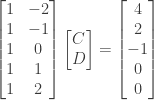
Answer: Assuming that the line in question has the form  the problem can be expressed as that of finding a solution to the system
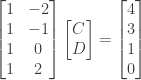
or  where
where  is the exact solution.
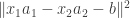
In this case there is no exact solution, so we look for the least squares solution  that minimizes the error vector
  . The error vector is minimized when it is orthogonal to the column space of
  and is therefore in the left nullspace of . We then have
  so that
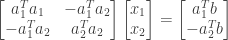
  is a solution to the system
  .
.
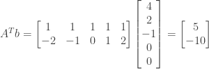
We have

and

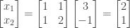
so that the system reduces to

or

expressed as a system of equations.
Multiplying the first equation by  and adding it to the second equation produces the system
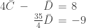
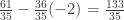
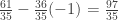
From the second equation we have  . Substituting that value into the first equation we have
  or
or  .
.
The line of best fit is therefore  .
.
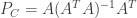
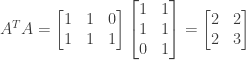
Given the matrix

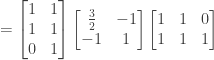
the projection matrix  onto the column space of can be computed as

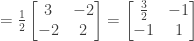
From above we have

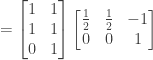
so that its inverse is
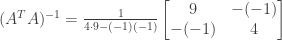

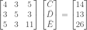
We then have


The projection of the vector onto the column space of is then


The vector  corresponds to the points on the least squares line of best fit
  for the times
  :
:


NOTE: This continues a series of posts containing worked out exercises from the (out of print) book Linear Algebra and Its Applications, Third Edition by Gilbert Strang.
If you find these posts useful I encourage you to also check out the more current Linear Algebra and Its Applications, Fourth Edition , Dr Strang’s introductory textbook Introduction to Linear Algebra, Fifth Edition
 and the accompanying free online course, and Dr Strang’s other books
 .
.


 ,
,  , and
, and  , and the two lines
  through the origin and
  through
  and
and  such that the distance
  between the points
  and
and  is at a minimum. Write down equations for
  when
when  ,
,  , and
, and  .
. with respect to
 and
and  we have
  (the inner product is the same no matter in which order we calculate it) and
  (the transpose of a difference is the same as the difference of the transposes). We then have


 ,
,  ,
,  ,
,  , and
, and  . The system of equations is then

 .
. that projects onto the row space of
  that projects onto the nullspace of
 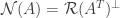 . Recall from exercise 3.3.11 that if
  and
and  a projection matrix onto
  then we have
  .
. or
or  .
. projects onto the column space of
  . We can then find the matrix that projects onto
  using the standard formula but substituting
 ![P_R = A^T[(A^T)^TA^T]^{-1}(A^T)^T = A^T(AA^T)^{-1}A](https://s0.wp.com/latex.php?latex=P_R+%3D+A%5ET%5B%28A%5ET%29%5ETA%5ET%5D%5E%7B-1%7D%28A%5ET%29%5ET+%3D+A%5ET%28AA%5ET%29%5E%7B-1%7DA&bg=ffffff&fg=333333&s=0&c=20201002)
 :
:
 .
.
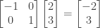
 and then substituting into the third equation we have
  . However we then get differing values of
  depending on whether we substitute into the second equation or the first. The system has no solution
  as written.
 . We have


 onto the line
  .
. is a basis for the subspace being projected onto, which is thus the column space of
 we have
 and
and

 is a vector with unit length. Show that the matrix
  (with rank 1) is a projection matrix.
 so that

 and
and  the rank-1 matrix
  geometrically. Why does
  ? (Give both a geometric and algebraic explanation.)
 produces
  . This can be thought of combining the following operations:
 ). Next, scale the resulting vector by a factor of 2 and reverse its direction (
 ). The resulting vector is still on the line onto which
  ). The final vector
  and the original vector


 this produces the vector
  :
:
 is applied again then it would reflect the vector

 and
and  . Find a nonzero vector


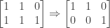
 by solving the system
  :
: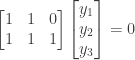
 and
and  are basic variables, and
  is a free variable. Setting
  we have
  (from the second row) and
  (from the first row). The vector
  is therefore a solution to

