I recently read the (excellent) online resource Quantum Computing for the Very Curious by Andy Matuschak and Michael Nielsen. Upon reading the proof that all length-preserving matrices are unitary and trying it out myself, I came to believe that there is an error in the proof as written, specifically with trying to show that off-diagonal entries in  are zero if
  is length-preserving.
Using the identity  , a suitable choice of
 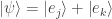 with
with  , and the fact that is length-preserving, Nielsen first shows that
  for .
for .
He then goes on to write “But what if we’d done something slightly different, and instead of using we’d used  ? … I won’t explicitly go through the steps – you can do that yourself – but if you do go through them you end up with the equation:
  .”
.”
I was an undergraduate physics and math major, but either I never worked with bra-ket notation and Hermitian conjugates or I’ve forgotten whatever I knew about them. In any case in working through this I could not get the same result as Nielsen; I simply ended up once again proving that .
After some thought and experimentation I concluded that the key is to choose 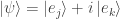 . Below is my (possibly mistaken!) attempt at a correct proof that all length-preserving matrices are unitary.
Proof: Let be a length-preserving matrix such that for any vector  we have
  . We wish to show that is unitary, i.e.,
  .
.
We first show that the diagonal elements of , or  , are equal to 1.
To do this we start with the unit vectors  and
and  with 1 in positions
  and
and  respectively, and 0 otherwise. The product
  is then the th column of , and
  is the
  th entry of or
  .
.
From the general identity  we also have
  . But since is length-preserving we have
  since is a unit vector.
We thus have  . So all diagonal entries of are 1.
We next show that the non-diagonal elements of , or with , are equal to zero.
Let with . Since is length-preserving we have

We also have where  . From the definition of the dagger operation and the fact that the nonzero entries of and have no imaginary parts we have
 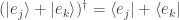 .
.
We then have


since we previously showed that all diagonal entries of are 1.
Since  and also
  we thus have for .
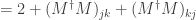
Now let with . Again we have  since is length-preserving, so that


Since  has an imaginary part for its (single) nonzero entry, in performing the dagger operation and taking complex conjugates we obtain
 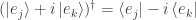 . We thus have


We also have


Since we have  or
or  so that .
But we showed above that . Adding the two equations the terms for  cancel out and we get
  for . So all nondiagonal entries of are equal to zero.
Since all diagonal entries of are equal to 1 and all nondiagonal entries of are equal to zero, we have and thus the matrix is unitary.
Since we assumed was a length-preserving matrix we have thus shown that all length-preserving matrices are unitary.


 is unitary.
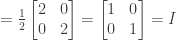
 is unitary if
  where
where  is the adjoint matrix to
  of
of  is symmetric we have
  and since the values of
  ) are all real we have
  . We thus have
 the matrix
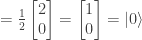
  is applied to a quantum state
  and then the outout is measured in the computational basis. Show that when the state
  is input to this circuit that the output is
  with probability 1, and that when the state
  is input to this circuit the output is
  with probability 1.
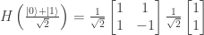
 .
. will produce the result 0 with probability
  and the value 1 with probability
  and
and  so the result will be
  , with the result
  . So the output as measured will always be
 , which when measured in the computational basis will always produce the value
 .
. (where
  and
and  are complex values) by the 2 by 2 matrix
  .
. and produces a two element column vector as a result, representing the output quantum state
  .
. from the left as
  . That produces another two-element column vector representing the final quantum state
  output from the quantum circuit.
 . Explain why
  would not make a suitable quantum gate by applying it to the quantum state
  .
.

 , verify that
  where
where  .
.


 of a set of
  values
  is usually expressed in terms of squared differences between those values and the mean
  of those values.
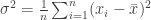
 between the values and the mean can also be expressed in term of the sum of squared pairwise differences
  among the values themselves, without reference to the mean
  .
. .
.![\sum_{i=1}^{n} \sum_{j=1}^{n} (x_i - x_j)^2 = \sum_{i=1}^{n} \sum_{j=1}^{n} [(x_i - \bar{x}) - (x_j - \bar{x})]^2](https://s0.wp.com/latex.php?latex=%5Csum_%7Bi%3D1%7D%5E%7Bn%7D+%5Csum_%7Bj%3D1%7D%5E%7Bn%7D+%28x_i+-+x_j%29%5E2+%3D+%5Csum_%7Bi%3D1%7D%5E%7Bn%7D+%5Csum_%7Bj%3D1%7D%5E%7Bn%7D+%5B%28x_i+-+%5Cbar%7Bx%7D%29+-+%28x_j+-+%5Cbar%7Bx%7D%29%5D%5E2&bg=ffffff&fg=333333&s=0&c=20201002)
![= \sum_{i=1}^{n} \sum_{j=1}^{n} [(x_i - \bar{x})^2 - 2 (x_i - \bar{x}) (x_j - \bar{x}) + (x_j - \bar{x})^2]](https://s0.wp.com/latex.php?latex=%3D+%5Csum_%7Bi%3D1%7D%5E%7Bn%7D+%5Csum_%7Bj%3D1%7D%5E%7Bn%7D+%5B%28x_i+-+%5Cbar%7Bx%7D%29%5E2+-+2+%28x_i+-+%5Cbar%7Bx%7D%29+%28x_j+-+%5Cbar%7Bx%7D%29+%2B+%28x_j+-+%5Cbar%7Bx%7D%29%5E2%5D&bg=ffffff&fg=333333&s=0&c=20201002)


 , the third term can be rewritten as
 . We can bring the difference
  out of the inner sum, since it does not depend on the index
 ![-2 \sum_{i=1}^{n} \sum_{j=1}^{n} (x_i - \bar{x}) (x_j - \bar{x}) = -2 \sum_{i=1}^{n} (x_i - \bar{x}) [\sum_{j=1}^{n} (x_j - \bar{x})]](https://s0.wp.com/latex.php?latex=-2+%5Csum_%7Bi%3D1%7D%5E%7Bn%7D+%5Csum_%7Bj%3D1%7D%5E%7Bn%7D+%28x_i+-+%5Cbar%7Bx%7D%29+%28x_j+-+%5Cbar%7Bx%7D%29+%3D+-2+%5Csum_%7Bi%3D1%7D%5E%7Bn%7D+%28x_i+-+%5Cbar%7Bx%7D%29+%5B%5Csum_%7Bj%3D1%7D%5E%7Bn%7D+%28x_j+-+%5Cbar%7Bx%7D%29%5D&bg=ffffff&fg=333333&s=0&c=20201002)
 can then be rewritten as
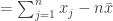
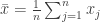 by definition, so we then have


 when
when  and
and  , we can consider only differences when
  (i.e., elements above the diagonal, if we consider the pairwise comparisons to form a matrix):
![= \frac{1}{2n} [\sum_{i < j} (x_i - x_j)^2 + \sum_{i = j} (x_i - x_j)^2 + \sum_{i > j} (x_i - x_j)^2]](https://s0.wp.com/latex.php?latex=%3D+%5Cfrac%7B1%7D%7B2n%7D+%5B%5Csum_%7Bi+%3C+j%7D+%28x_i+-+x_j%29%5E2+%2B+%5Csum_%7Bi+%3D+j%7D+%28x_i+-+x_j%29%5E2+%2B+%5Csum_%7Bi+%3E+j%7D+%28x_i+-+x_j%29%5E2%5D&bg=ffffff&fg=333333&s=0&c=20201002)
![\frac{1}{2n} [\sum_{i < j} (x_i - x_j)^2 + 0 + \sum_{i < j} (x_i - x_j)^2]](https://s0.wp.com/latex.php?latex=%5Cfrac%7B1%7D%7B2n%7D+%5B%5Csum_%7Bi+%3C+j%7D+%28x_i+-+x_j%29%5E2+%2B+0+%2B+%5Csum_%7Bi+%3C+j%7D+%28x_i+-+x_j%29%5E2%5D&bg=ffffff&fg=333333&s=0&c=20201002)
![\frac{1}{2n} [2 \sum_{i < j} (x_i - x_j)^2] = \frac{1}{n} \sum_{i < j} (x_i - x_j)^2](https://s0.wp.com/latex.php?latex=%5Cfrac%7B1%7D%7B2n%7D+%5B2+%5Csum_%7Bi+%3C+j%7D+%28x_i+-+x_j%29%5E2%5D+%3D+%5Cfrac%7B1%7D%7Bn%7D+%5Csum_%7Bi+%3C+j%7D+%28x_i+-+x_j%29%5E2&bg=ffffff&fg=333333&s=0&c=20201002)
![= \frac{1}{n} [\frac{1}{n} \sum_{i < j} (x_i - x_j)^2]](https://s0.wp.com/latex.php?latex=%3D+%5Cfrac%7B1%7D%7Bn%7D+%5B%5Cfrac%7B1%7D%7Bn%7D+%5Csum_%7Bi+%3C+j%7D+%28x_i+-+x_j%29%5E2%5D&bg=ffffff&fg=333333&s=0&c=20201002)

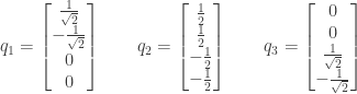
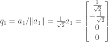
 and the following vectors
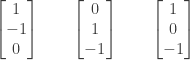
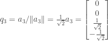
 and normalize it to create
  :
:

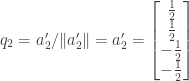
 and create a second orthogonal vector
  by subtracting from
  its projection on
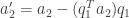
![= a_2 - \left[ \frac{1}{\sqrt{2}} \cdot 0 + (-\frac{1}{\sqrt{2}}) \cdot 1 + 0 \cdot (-1) \right]q_1 = a_2 - (-\frac{1}{\sqrt{2}})q_1 = a_2 + \frac{1}{\sqrt{2}}q_1](https://s0.wp.com/latex.php?latex=%3D+a_2+-+%5Cleft%5B+%5Cfrac%7B1%7D%7B%5Csqrt%7B2%7D%7D+%5Ccdot+0+%2B+%28-%5Cfrac%7B1%7D%7B%5Csqrt%7B2%7D%7D%29+%5Ccdot+1+%2B+0+%5Ccdot+%28-1%29+%5Cright%5Dq_1+%3D+a_2+-+%28-%5Cfrac%7B1%7D%7B%5Csqrt%7B2%7D%7D%29q_1+%3D+a_2+%2B+%5Cfrac%7B1%7D%7B%5Csqrt%7B2%7D%7Dq_1&bg=ffffff&fg=333333&s=0&c=20201002)

 :
:

 and attempt to create another orthogonal vector
  by subtracting from
  its projections on
![= a_3 - \left[ \frac{1}{\sqrt{2}} \cdot 1 + (-\frac{1}{\sqrt{2}}) \cdot 0 + 0 \cdot (-1) \right]q_1- \left[ \frac{1}{\sqrt{6}} \cdot 1 + \frac{1}{\sqrt{6}} \cdot 0 + (-\frac{2}{\sqrt{6}}) \cdot (-1) \right] q_2](https://s0.wp.com/latex.php?latex=%3D+a_3+-+%5Cleft%5B+%5Cfrac%7B1%7D%7B%5Csqrt%7B2%7D%7D+%5Ccdot+1+%2B+%28-%5Cfrac%7B1%7D%7B%5Csqrt%7B2%7D%7D%29+%5Ccdot+0+%2B+0+%5Ccdot+%28-1%29+%5Cright%5Dq_1-+%5Cleft%5B+%5Cfrac%7B1%7D%7B%5Csqrt%7B6%7D%7D+%5Ccdot+1+%2B+%5Cfrac%7B1%7D%7B%5Csqrt%7B6%7D%7D+%5Ccdot+0+%2B+%28-%5Cfrac%7B2%7D%7B%5Csqrt%7B6%7D%7D%29+%5Ccdot+%28-1%29+%5Cright%5D+q_2&bg=ffffff&fg=333333&s=0&c=20201002)


 we cannot create a third orthogonal vector to
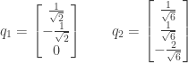
 ,
,  . Thus only
 that form an orthonormal basis for the subspace.


![= a_2 - \left[ \frac{1}{\sqrt{2}} \cdot 0 + (-\frac{1}{\sqrt{2}}) \cdot 1 + 0 \cdot (-1) + 0 \cdot 0 \right]q_1 - \left[ 0 \cdot 0 + 0 \cdot 1 + \frac{1}{\sqrt{2}} \cdot (-1) + (-\frac{1}{\sqrt{2}}) \cdot 0 \right]q_3](https://s0.wp.com/latex.php?latex=%3D+a_2+-+%5Cleft%5B+%5Cfrac%7B1%7D%7B%5Csqrt%7B2%7D%7D+%5Ccdot+0+%2B+%28-%5Cfrac%7B1%7D%7B%5Csqrt%7B2%7D%7D%29+%5Ccdot+1+%2B+0+%5Ccdot+%28-1%29+%2B+0+%5Ccdot+0+%5Cright%5Dq_1+-+%5Cleft%5B+0+%5Ccdot+0+%2B+0+%5Ccdot+1+%2B+%5Cfrac%7B1%7D%7B%5Csqrt%7B2%7D%7D+%5Ccdot+%28-1%29+%2B%C2%A0+%28-%5Cfrac%7B1%7D%7B%5Csqrt%7B2%7D%7D%29+%5Ccdot+0+%5Cright%5Dq_3&bg=ffffff&fg=333333&s=0&c=20201002)